


-
The safe production of coal chemistry processes directly relates to national energy security, and coal gasification technology is the core unit of modern coal chemistry; its safety is crucial. Coal gasification technology has characteristics such as high temperature and high pressure, etc. The process system is complex, and the safety risk is high[1]. During coal gasification, coal is converted into syngas, which primarily consists of carbon monoxide and hydrogen and which has a wide range of applications as a common raw material in industry[2,3]. However, syngas is flammable, explosive, and toxic due to its chemical compositional[4]. Once leakage occurs, it can easily cause poisoning, asphyxiation, fire, or explosions, posing serious threats to the safety of personnel, equipment, facilities, and the surrounding environment. Compared to other components prone to leakage, the coal gasification syngas outlet pipelines is at a greater risk of leakage due to its long operational cycle and vulnerability to external environmental factors. Therefore, conducting a risk assessment for coal gasification syngas pipelines is essential to prevent accidents and minimize leakage risks.
In terms of risk assessment of coal gasification in the coal chemical industry, Liu et al. applied the Similarity Aggregation Method (SAM) based on Bayesian Networks (BN) and trapezoidal intuitionistic fuzzy numbers to evaluate the risk assessment of coal gasification and identify weak points[5]. To compensate for the lack of failure data in the gasification system, Liu et al. proposed a Dynamic Bayesian Network (DBN) integrated with Monte Carlo simulation to assess the reliability of the coal gasification locking drum valving system[6]. Li et al. utilized text mining (TM) technology to develop an enhanced method for identifying safety risk factors from a large number of coal chemical industry accident reports; this method introduces a new strategy for improving safety decision-making in coal chemical industries, thereby aiding in accident prevention[7]. Sun et al. combined key events and safety barriers to propose a methodology for control of coal gasification process hazards, it includes identifying process hazards through key events, evaluating protection performance using barrier maps, and quantifying hazard factors using BN[1].
In the study of syngas pipeline leakage, current research primarily focuses on the analyzing the causes of leakage and potential countermeasures. Li et al. conducted a flange leakage analysis for a crude syngas pipeline with a pipeline classification of GC1 using both equivalent pressure and stress calculation methods[8]. Most current research focuses on the coal gasification process or system failures, with limited studies on the assessment of syngas leakage risk. Additionally, most risk assessment methods in the coal chemical industry rely on static analysis, which fails to capture the dynamic evolution of risk factors over time. BNs are more flexible and efficient than traditional risk assessment methods such as Hazard and Operability Analysis (HAZOP), Fault Tree Analysis (FTA), Event Tree Analysis (ETA), and BT, and are widely applied in industrial process risk analysis[9−11]. Khakzad et al. mapped a bow-tie model to a BN to enable quantitative analysis of dynamic risk in process systems[12]. Guo et al. proposed an improved SAM-based Fuzzy Bayesian Network (FBN) method to better handle type uncertainty, which makes the tank prediction more realistic and reliable[13]. Fan et al. developed a quantitative BN-based risk analysis model to analyze the toxicity and flammability risks of ammonia during ship-to-ship fueling, accomplishing an accurate quantification of ammonia fueling risks[14]. Wang et al. investigated a risk evaluation model based on BN for polar drilling operations, providing effective preventive strategies[15]. Traditional BN methods have static limitations and cannot describe the dynamic change evolution of the system. To address this problem, DBN have been proposed and integrated with other risk assessment methods to provide dynamic support for risk warning, security prevention, and control. Wang proposed a dynamic risk analysis approach based on Dynamic Bow-Tie (DBT) and DBN to obtain the dynamic change features of incident scenarios involving heating furnace oil and gas leakage faults as the research object[16]. Xu investigated a dynamic risk analysis method for underground gas storage processes and established a corresponding evaluation model, offering practical value for enhancing the safety of such facilities[17]. Wang & Zhang proposed a DBN-based hydrogen leakage risk evaluation method for HECS, providing a theoretical basis for accident prevention and routine care[18]. Given the complexity of conveyor belts in power plants, Liu et al. proposed a BT and uncertainty fuzzy DBN risk assessment method for coal conveyor belts, offering a scientific basis for their safety control[19].
To this end, a risk assessment approach based on DBN for syngas pipeline leakage in coal gasification is proposed in this study. Using syngas pipeline leakage in coal gasification as the research object, a risk analysis model is developed based on BT analysis methodology. The model is transformed into a DBN using a mapping algorithm. To quantify prior probabilities, fuzzy set theory, improved similarity aggregation techniques, and expert judgment are employed. Additionally, a Leaky Noisy-or gate model is introduced to better address the inherent inconclusiveness in DBN. Predicting the dynamic probability of a syngas pipeline leakage occurring and the probability of potential consequences by adding time series.
-
The Bow-Tie (BT) model consists of two components: the Fault Tree (FT) and the Event Tree (ET), which systematically analyze accident causes and their developmental consequences. This model has been widely applied in risk analysis, particularly within the domain of chemical safety[20]. Specifically, FTA is used to identify and analyze hazard sources, whereas ETA is used to describe the evolution of events following a risk occurrence. The BT model clearly shows the evolutionary logic of an event and combines the advantages of FTA and ETA, thereby visually presenting both the causes and development process of an accident.
Dynamic Bayesian Network
Theoretical
-
DBN is a time series extension of BN that combines Bayesian theorem with chain rules and describes the dynamic evolution over time through introducing HMM (Hidden Markov Model)[21,22]. The analysis of the system state over time is achieved by adding time-slice dependencies to the topology of the original static Bayesian network. In DBN modeling, time slice is an important concept. The node state of the current time slice is affected by its parent nodes and previous time slice nodes, enabling DBN to effectively capture dynamic changes in complex systems.
The transfer probability is calculated as follows:
$ P({X_t}|{X_{t{\text{ - }}1}}) = \prod\limits_{i = 1}^n {P(X_t^i|{P_a}(X_t^i))} $ (1) where,
$ X_t^i $ $ {P_a}(X_t^i) $ Structural building
-
Based on the mapping algorithm, the BT model evolved after the leakage of a syngas pipeline is transformed into a DBN. The basic events in the BT model are mapped to basic events in the DBN, middle events to middle nodes, top events to leaf nodes, safety barriers to barrier nodes, consequences of accidents to consequence nodes, and logic gate relationships to conditional probability tables (CPT)[23].
Prior probability calculation
-
Due to the absence of a well-established failure database in China, the expert scoring method was employed for probabilistic assessment. Experts from relevant industry sectors were consulted to assess the occurrence probabilities of basic events. As experts cannot precisely quantify the probabilities of event occurrences, an improved SAM method was used to summarize the expert opinions and fuzzy set theory was subsequently applied to refine the data. The expert panel comprised five technical professionals from relevant industries, with background information collected on their education background, titles, and years of service. In this study, seven linguistic terms are used to describe the occurrence probability of basic events: 'very low (VL)', 'low (L)', 'mid-to-low (ML)', 'medium (M)', 'mid-to-high (MH)', 'high (H)', and 'very high (VH)'.
Expert language conversion to fuzzy numbers
-
The expert panel risk assessment opinions on the basic events are translated into intuitional fuzzy numbers, as shown in Table 1.
Table 1. Transformation of expert opinion into fuzzy numbers.
Natural language terms and codes Fuzzy intervals (a, b, c, d) VL (0, 0, 0.1, 0.2) L (0.1, 0.2, 0.2, 0.3) ML (0.2, 0.3, 0.4, 0.5) M (0.4, 0.5, 0.5, 0.6) MH (0.5, 0.6, 0.7, 0.8) H (0.7, 0.8, 0.8, 0.9) VH (0.8, 0.9, 1, 1) Determination of expert weights
-
Based on the scoring rules for education level, title, and length of service, as shown in Table 2, the proportion of each expert's score relative to the total score of all experts is calculated to obtain the weights of the experts.
Table 2. Rules for scoring the importance of experts.
Factor Grade Weight Title Professor/Chief engineer 5 Associate Professor/Senior engineer 4 Lecturer/Engineer 3 Technician 2 Laborer 1 Educational background Doctoral degree 5 Master's degree 4 Bachelor's degree 3 Senior high school 2 Junior high school and below 1 Years of service > 20 years 5 15−20 years 4 10−15 years 3 5−10 years 2 < 5 years 1 Fuzzy number aggregation
-
Due to potential discrepancies among expert opinions, SAM is used to aggregate expert opinions and ensure consistency. SAM is a method proposed by Hsu & Chen to deal with group resolutions, which can be effective in processing expert group opinions with exact values[24]. Guo et al. proposed an improved SAM that accounts for individual differences among experts, thereby enhancing the accuracy and reliability of the aggregated results[13]. Therefore, this study uses the improved SAM to aggregate the judgments of different experts into intuitionistic fuzzy numbers.
① Calculate the degree of agreement of each expert judgment pair. The two sets of expert judgments are Ai = (a1, a2, a3, a4), Aj = (b1, b2, b3, b4), then the degree of agreement between the two pairs of expert opinions is:
$ S({\tilde A_i},{\tilde A_j}) = 1 - \dfrac{1}{4}\sum\nolimits_{i = 1}^4 {\left| {{a_i} - \left. {{b_i}} \right|} \right.} $ (2) when Ai = Aj, S (Ai, Aj) = 1, indicating that the two groups of experts have the same opinion.
② Calculate the expert's absolute agreement
$ WA({E_i}) = \dfrac{{\displaystyle\sum\nolimits_ {{\begin{aligned} &j = 1 \\[-5pt] &j \ne i \end{aligned}}} ^5 {W({E_j}) \times S({A_i},{A_j})} }}{{\displaystyle\sum\nolimits_ {{\begin{aligned} & j = 1 \\[-5pt] & j \ne i \end{aligned}}} ^5 {W({E_j})} }} $ (3) where, S (Ai, Aj) is the degree of agreement between the opinions of the ith and jth experts, W(Ej) is the weight of the jth (j = 1, 2, ... , 5, except i) of the experts' weights.
③ Calculate the expert's degree of relative consistency.
$ RA({E_i}) = \dfrac{{WA({E_i})}}{{\displaystyle\sum\nolimits_{i = 1}^5 {WA({E_i})} }} $ (4) where, WA(Ei) is the absolute agreement of the ith expert.
④ Calculate the degree of experts' consensus coefficient (CC).
$ CC({E}_{i})=\beta \times W({E}_{i})+(1-\beta )\times RA({E}_{i}) $ (5) where, W(Ei) is the weight of the ith expert and RA(Ei) is the relative consistency of the ith expert. β (0 ≤ β ≤ 1) is defined as a relaxation factor, with larger β indicating greater importance of expert weights and smaller β indicating greater importance of expert relative consistency[5].
⑤ The aggregated expert opinions were used to derive the overall fuzzy number R.
$ \tilde R = CC({E_1}) \times {\tilde A_1} + CC({E_2}) \times {\tilde A_2} + \cdot \cdot \cdot + CC({E_5}) \times {\tilde A_5} $ (6) where, CC(Ei) is the consensus coefficient of the ith expert and Ai is the number of fuzzy opinions of the ith expert (i = 1, 2, ... , 5).
Defuzzification
-
The fuzzy number obtained by aggregation must also be converted into a fuzzy possibility number FPS. There are many ways of defuzzification method, this study uses the centroid method[25]. For a fuzzy number R = (a1, a2, a3, a4), there is:
$ \begin{split} FPS =\;& \dfrac{{\int_{{a_1}}^{{a_{_2}}} {\dfrac{{x - {a_1}}}{{{a_2} - {a_1}}}xdx{\text{ + }}\int_{{a_{\text{2}}}}^{{a_{\text{3}}}} {xdx{\text{ + }}} \int_{{a_{\text{3}}}}^{{a_{_{\text{4}}}}} {\dfrac{{{a_{\text{4}}} - x}}{{{a_4} - {a_3}}}xdx} } }}{{\int_{{a_1}}^{{a_{_2}}} {\dfrac{{x - {a_1}}}{{{a_2} - {a_1}}}dx{\text{ + }}\int_{{a_{\text{2}}}}^{{a_{\text{3}}}} {dx{\text{ + }}} \int_{{a_{\text{3}}}}^{{a_{_{\text{4}}}}} {\dfrac{{{a_{\text{4}}} - x}}{{{a_4} - {a_3}}}dx} } }} \\ =\;& \dfrac{1}{3}\dfrac{{{{({a_4} + {a_3})}^2} - {a_4}{a_3} - {{({a_1} + {a_2})}^2} + {a_1}{a_2}}}{{({a_4} + {a_3} - {a_1} - {a_2})}} \end{split} $ (7) Calculation of fuzzy failure probability
-
To correspond the fuzzy failure probability to the intuitionistic fuzzy probability interval, the FPS was converted to FFP using the conversion formula proposed by Onisawa[26].
$ FFP = \left\{\begin{array}{ll} 1/10^K & FPS \ne 0\\ 0 & FPS=0\end{array}\right. \; K = {\left[ {\left( {\dfrac{{1 - FPS}}{{FPS}}} \right)} \right]^{\frac{1}{3}}} \times 2.301 $ (8) Fuzzy set theory
-
In 1965, Prof. Zadeh[27] pioneered the development of fuzzy set theory, introducing the concept of an affiliation function and laying the foundation for fuzzy mathematics. In a fuzzy set, elements are not only expressed by 0 and 1 but can also take any real number between [0,1], thus describing the fuzziness and uncertainty more precisely[28]. A trapezoidal fuzzy number is selected as the affiliation function in this paper. The trapezoidal fuzzy number consists of four parameters (a, b, c, d), and its affiliation function is defined as follows:
$ \mu \tilde A(x) = \left\{ \begin{array}{ll} 0 &(x \lt a) \\ \dfrac{{x - a}}{{b - a}} &(a \lt x \leqslant b) \\ 1 &(b \lt x \leqslant c) \\ \dfrac{{d - x}}{{d - c}} &(c \lt x \leqslant d) \\ 0 &(d \lt x) \end{array} \right. $ (9) Leaky Noisy-or gate model
-
In traditional DBN models, conditional probabilities are usually transformed through logic gates; this method is too absolute in determining conditional probabilities and describes only simple binary states. In reality, humans may overlook specific potential nodes when identifying risks, which can still exert influence on outcome nodes.
Based on this realization, the concept of omission probability was first proposed by Henrion[29], and subsequently, Li et al.[30] and Oniśko et al.[31] further developed the Leaky Noisy-or gate extension model based on it. To correct the conditional probability, the Leaky Noisy-or gate model is added, where the missing nodes are denoted by XL.
Suppose the child node Y has only two root nodes XL and XALL, where XALL represents the sum of all elements except XL, and their corresponding probabilities are PL and PALL, respectively, we have:
$ P(Y|{X_L}) = 1 - (1 - {P_L})(1 - {P_{all}}) = {P_L} + {P_{all}} - {P_L}{P_{all}} $ (10) $ P(Y|\bar X) = {P_{all}} $ (11) Associating the above equations yields Eqn (12):
$ {P_i} = \dfrac{{P(Y|{X_L}) - P(Y|\bar X)}}{{1 - P(Y|\bar X)}} $ (12) The connection probabilities of all the root nodes of the child node Y can be calculated from Eq (12). Let the connection probability of XL be PL = 0.01, The conditional probability of the child node Y can then be calculated.
$ P(Y) = 1 - (1 - {P_L}){\prod\nolimits _{i:{X_i} \in {X_p}}}(1 - {P_i}) $ (13) State transfer probability table
-
Time-dependent events, such as corrosion, wear, etc., are selected as dynamic basic events. The Weibull distribution, being more appropriate for describing failure behavior than the normal distribution, and hence, it is chosen as the life cycle distribution to represent the failure probability[32].
A two-parameter Weibull distribution is used to calculate the state transfer probability of dynamic nodes in the DBN, where η is the scale parameter, and β is the shape parameter, obtaining parameters based on literature search[33]. The transfer probability is calculated as follows:
$ \begin{aligned} \left\{ \begin{array}{l} P(Pa({X_{t + \Delta t}}) = T|Pa({X_t}) = T) = 1\\ P(Pa({X_{t + \Delta t}}) = N|Pa({X_t}) = N) = {e^{{{\left( {\frac{t}{\eta }} \right)}^\beta } - {{\left( {\frac{{t + \Delta t}}{\eta }} \right)}^\beta }}} \end{array} \right. \end{aligned} $ (14) where P(Pa(Xt+Δt) = T|Pa(Xt) = T) denotes the probability that when node Pa(Xt) occurs on segment t, Pa(Xt + Δt) also occurs on segment t as well. P(Pa(Xt + Δt) = N|Pa(Xt) = N denotes the probability that when node Pa(Xt) does not occur on segment t, Pa(Xt + Δt) also does not occur on segment t.
-
Hazard identification is the most fundamental task in conducting a risk analysis, which includes identifying the risk factors that may lead to leaks and the types of potential accidents. Based on accident cases, enterprise anomaly reports, and literature research, the risk factors contributing to syngas pipeline leakage at the coal gasification outlet were identified and systematically categorized. These risk factors are broadly categorized into human factors, equipment factors, and environmental factors.
The human factor, an important exogenous factor leading to accidents, are particularly prominent in safety incidents such as pipeline leaks. Inaccurate judgment or poor decision-making by personnel, which impairs hazard recognition during operations, is a common contributing factor to accidents. The equipment factor primarily divide leaks in syngas outlet lines into two parts: body leaks and associated accessory leaks.
The occurrence of leaks is highly dependent on the characteristics of the syngas, operational environments, and process conditions. Environmental factors also play a crucial role, as extreme weather or unexpected conditions can damage pipelines and lead to leaks.
Syngas, the product of the gasification reaction, is highly flammable and explosive. Once leaked and exposed to an ignition source, it can readily trigger a fire or explosion. Therefore, in the event of a syngas pipeline leak in coal gasification, it is crucial to rely on multiple safety barriers, including monitoring and alarms, emergency response, emergency shutdown, immediate ignition, restricted space, delayed ignition, to prevent escalation, and avert catastrophic consequences. Different combinations of safety barrier failures can lead to varied accident consequences. Consequential events include safety, safety proliferation, jet fire, flash fire, poisoning asphyxiation, and vapor cloud explosion. The monitoring and alarm barrier continuously monitors parameter changes and promptly triggers alerts upon detecting anomalies. Monitoring and alarm are crucial for the early detection and control of accidents. Upon receiving an alarm, the emergency response barrier is immediately activated to facilitate a quick response and judgment, thereby slowing down the further development of the accident. Emergency shutdown barriers facilitate the timely cessation of operations during a syngas leak, thereby preventing accident escalation. If these barriers fail, the leaking syngas may encounter an ignition source and ignite immediately, resulting in a jet fire accident and jeopardizing the safety of both equipment and personnel. In confined spaces, large volumes of leaked syngas can accumulate. If ignited, this may cause a vapor cloud explosion, resulting in extensive damage to the facility and potential loss of life. In unconfined spaces, ignition of leaked syngas may result in a flash fire. Although the flame spreads rapidly, the associated hazard is relatively small because there is no significant explosive shock wave. If a syngas leak is not ignited and continues to disperse in a confined space, the concentration of CO will gradually rise. As CO is colorless, odorless, and non-irritating, it can cause unnoticed poisoning of personnel, and in severe cases, can lead to death by asphyxiation.
Combining identified risk factors and accident types associated with safety barriers, a BT model of the post-leakage evolution of the syngas pipeline is drawn, as shown in Fig. 1. Basic events are denoted by X and middle node events are denoted by M. Table 3 presents information about one top event, 16 middle events, and six consequence events, while Table 4 presents information on 39 basic events. Table 5 presents information about six security barriers.
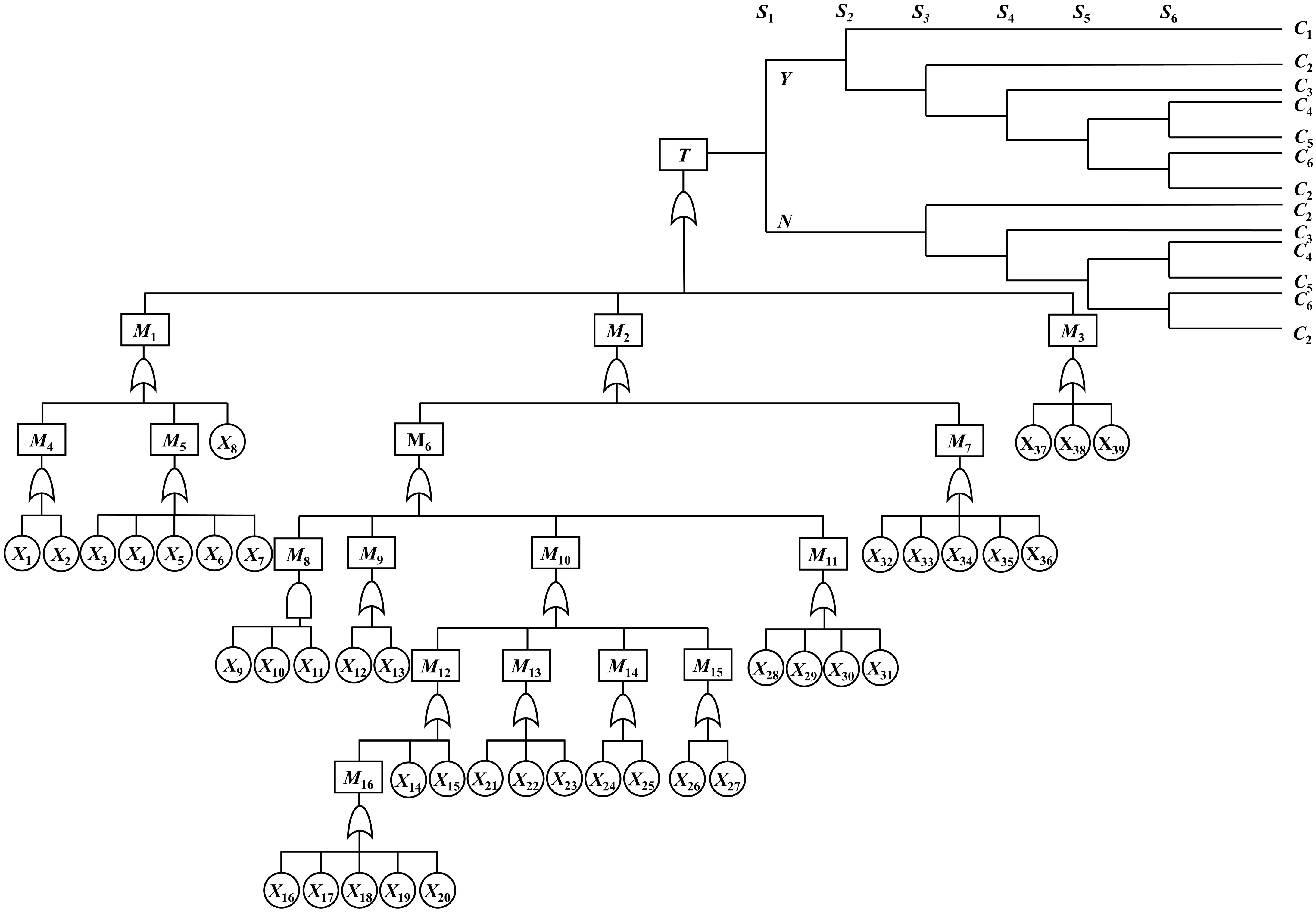
Figure 1.
Syngas pipeline leak BT model.
Table 3. Top, middle, and consequence events in the BT model.
Code name Descriptive Code name Descriptive T Gasifier syngas pipeline leakage M12 Low liquid level in the cooling chamber M1 Human factors M13 Furnace temperature increase M2 Equipment factors M14 Burn-through of drop tube M3 Environmental factor M15 Clogged pipes M4 Lack of safety awareness M16 Low flow rate of cooling water M5 Error of judgment C1 Security M6 Syngas pipeline leakage C2 Security proliferation M7 Leakage of related accessories C3 Jet fire M8 Pipeline corrosion C4 Vapor cloud explosion M9 Pipe erosion and wear C5 Flash fire M10 Pipe overheating C6 Poisoning asphyxiation M11 Pipe quality defects Table 4. Basic events in the BT model and the corresponding prior and posterior probabilities.
Code name Descriptive Prior probability Posterior probability X1 Insufficient operational experience 2.4594 × 10⁻³ 6.9466 × 10−3 X2 Inadequate pre-service training 4.1776 × 10⁻³ 1.2228 × 10−2 X3 Inadequate inspection 7.5334 × 10⁻³ 2.5832 × 10−2 X4 Quality control is not strict 8.0194 × 10⁻³ 2.4290 × 10−2 X5 Inspection and disassembly is not strict 9.4218 × 10⁻³ 3.2870 × 10−2 X6 Emergency response not in place 2.2802 × 10⁻³ 7.7090 × 10−3 X7 Operational errors 3.7668 × 10⁻³ 1.0847 × 10−2 X8 Third party destruction 1.1149 × 10⁻⁴ 4.0252 × 10−4 X9 Failure of corrosion protection layer 3.6306 × 10⁻³ 3.6320 × 10−3 X10 Corrosive media 1.2773 × 10⁻² 1.2775 × 10−2 X11 Stress corrosion 1.0382 × 10⁻² 1.0383 × 10−2 X12 High coal ash content 1.2346 × 10⁻³ 4.2221 × 10−3 X13 Syngas carries water flushing 3.7584 × 10⁻³ 1.0209 × 10−2 X14 Malfunction of black water regulating valve 1.1120 × 10⁻² 2.8586 × 10−2 X15 Severe water carryover of process gas 3.9371 × 10⁻³ 9.5605 × 10−3 X16 Abnormalities in the cooling pump 6.6038 × 10⁻³ 1.5291 × 10−2 X17 Blackwater filter clogged 1.3997 × 10⁻² 3.1299 × 10−2 X18 Clogging of the cooling ring 9.3452 × 10⁻³ 1.7828 × 10−2 X19 Clogged make-up water pipe 7.6128 × 10⁻³ 1.2786 × 10−2 X20 Abnormality of cooling water regulating valve 9.3608 × 10⁻³ 2.1401 × 10−2 X21 Coal line line breaks 1.4587 × 10⁻³ 4.4175 × 10−3 X22 Oxygen regulator valve failure 2.4594 × 10⁻³ 5.7867 × 10−3 X23 Coal quality change 4.1820 × 10⁻³ 9.0992 × 10−3 X24 Slag hanging on the descending pipe 3.2415 × 10⁻³ 8.7956 × 10−3 X25 Deformation of the cooling ring 4.6277 × 10⁻³ 1.3752 × 10−2 X26 Internal scaling 4.4655 × 10⁻³ 1.2345 × 10−2 X27 Foreign body blockage 2.1168 × 10⁻³ 4.5925 × 10−3 X28 Design defects 9.0316 × 10⁻⁴ 1.9623 × 10−3 X29 Welding defects 1.0935 × 10⁻² 3.1067 × 10−2 X30 Improper material 7.7409 × 10⁻³ 1.74125 × 10−2 X31 Life limitation 3.0448 × 10⁻³ 6.6177 × 10−3 X32 Gasket failure 8.6622 × 10⁻³ 4.0003 × 10−2 X33 Seal failure 8.9526 × 10⁻³ 3.9465 × 10−2 X34 Flange scouring and wear 1.0531 × 10⁻² 5.0083 × 10−2 X35 Valve scouring and wear 4.0810 × 10⁻³ 1.9578 × 10−2 X36 Accessory deterioration 2.7119 × 10⁻³ 1.1904 × 10−2 X37 Typhoon 5.6502 × 10⁻⁶ 6.1817 × 10−6 X38 Earthquake 4.0054 × 10⁻⁵ 5.1756 × 10−5 X39 Other natural disasters 4.0054 × 10⁻⁵ 8.3535 × 10⁻⁵ Table 5. Prior probability of safety barrier failure.
Code name Descriptive Prior probability S1 Monitoring alarms 6.0844 × 10⁻³ S2 Emergency response 2.8469 × 10⁻³ S3 Emergency shutdown 3.4036 × 10⁻³ S4 Immediate ignition 3.6761 × 10⁻³ S5 Delayed ignition 2.5638 × 10⁻³ S6 Restricted space 1.5784 × 10⁻³ BT maps to DBN
-
Based on the mapping algorithm, the evolved BT model following syngas pipeline leakage is converted into a Bayesian network. The resulting DBN model for syngas leakage is shown in Fig. 2.
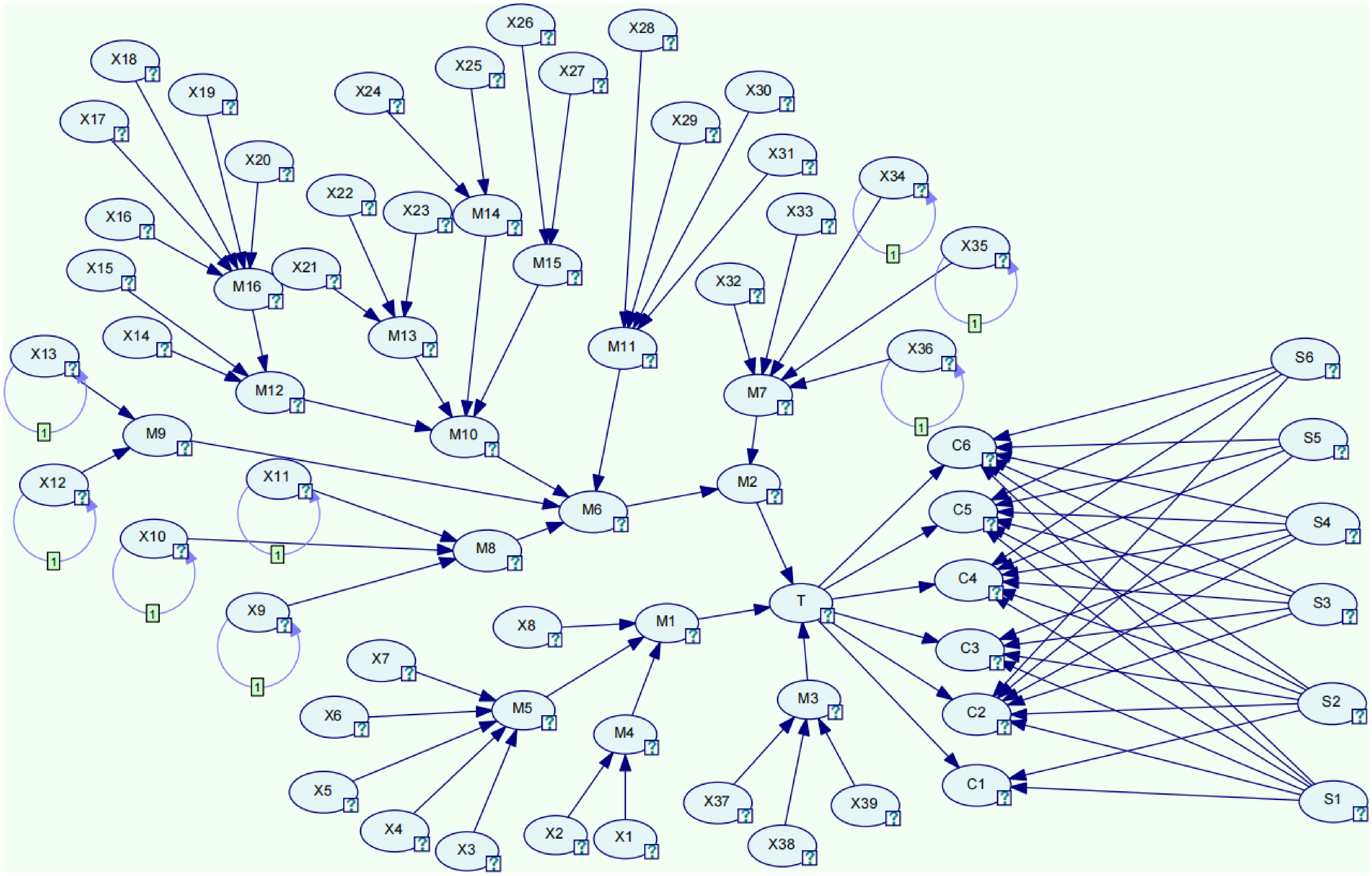
Figure 2.
Bayesian structure chart.
Bayesian network parameter learning
Prior probability calculation
-
As an example, the calculation of the a priori probability for operational error in basic event X7 is presented, with the detailed process shown in Table 6.
Table 6. X7 detailed calculation process.
Natural language (L, M, MH, M, M) $ W({E_i}) $ $ W({E_1}) = \dfrac{{5 + 5 + 3}}{{51}} = 0.255 $ $ \begin{gathered}W(E_1)=0.255;\ W(E_2)=0.235; \\ W(E_3)=0.137;\ W(E_4)=0.137; \\ W(E_5)=0.235 \\ \end{gathered} $ $ S({\tilde A_i},{\tilde A _j}) $ $ \begin{gathered} S({\tilde A _{\text{1}}},{\tilde A _{\text{2}}}) = 1 - \dfrac{1}{4}\sum\nolimits_{i = 1}^4 {\left| {{a_i} - \left. {{b_i}} \right|} \right.} = 1 - \dfrac{1}{4}(0.3 + 0.3 + 0.3 + 0.3) = 0.7 \end{gathered} $ $ \begin{gathered}S(\tilde{A}_{\text{1}},\tilde{A}_{\text{2}})\text{ = 0}\text{.70};\ S(\tilde{A}_{\text{1}},\tilde{A}_{\text{3}})\text{ = 0}\text{.55}; \\ S(\tilde{A}_{\text{1}},\tilde{A}_{\text{4}})\text{ = 0}\text{.70};\ S(\tilde{A}_{\text{1}},\tilde{A}_{\text{5}})\text{ = 0}\text{.70}; \\ ....... \\ \end{gathered} $ $ WA({E_i}) $ $ \begin{aligned} WA({E_{\text{1}}}) =\;& \dfrac{{\displaystyle\sum\nolimits_{{\begin{aligned} j = 1 \\[-5pt] j \ne i \end{aligned}}} ^5 {W({E_j}) \times S({A_i},{A_j})} }}{{\displaystyle\sum\nolimits_{{\begin{aligned} j = 1 \\[-5pt] j \ne i \end{aligned}}} ^5 {W({E_j})} }} = \dfrac{{{\text{0}}{\text{.235}} \times {\text{0}}{\text{.7 + 0}}{\text{.137}} \times {\text{0}}{\text{.55 + 0}}{\text{.137}} \times {\text{0}}{\text{.7 + 0}}{\text{.235}} \times {\text{0}}{\text{.7}}}}{{{\text{0}}{\text{.235 + 0}}{\text{.137 + 0}}{\text{.137 + 0}}{\text{.235}}}} \\ =\;& 0{\text{.6724}} \end{aligned} $ $ \begin{gathered} WA({E_{\text{1}}}) = {\text{0}}{\text{.67238}}; \\ WA({E_{\text{2}}}) = {\text{0}}{\text{.87297}}; \\ WA({E_{\text{3}}}) = {\text{0}}{\text{.76125}}; \\ WA({E_{\text{4}}}) = {\text{0}}{\text{.88741}};\\ WA({E_{\text{5}}}) = {\text{0}}{\text{.87297}} \end{gathered} $ $ RA({E_i}) $ $ \begin{aligned} RA({E_{\text{1}}}) =\;& \dfrac{{WA({E_{\text{1}}})}}{{\displaystyle\sum\nolimits_{i = 1}^5 {WA({E_i})} }} {\text{ = }}\dfrac{{{\text{0}}{\text{.6724}}}}{{{\text{0}}{\text{.67238 + 0}}{\text{.87297 + 0}}{\text{.76125 + 0}}{\text{.88741 + 0}}{\text{.87297}}}} = \dfrac{{{\text{0}}{\text{.67240}}}}{{4.06698}} \\=\;& 0.1653 \end{aligned} $ $ \begin{gathered} RA({E_{\text{1}}}) = {\text{0}}{\text{.1653}}; \\ RA({E_{\text{2}}}) = {\text{0}}{\text{.2146}}; \\ RA({E_{\text{3}}}) = {\text{0}}{\text{.1872}}; \\ RA({E_{\text{4}}}) = {\text{0}}{\text{.2182}}; \\ RA({E_{\text{5}}}) = {\text{0}}{\text{.2146}} \end{gathered} $ $ CC({E_i}) $ $ \begin{array}{c}CC({E}_{1})=\beta \times W({E}_{1})\text{+}({1-}\beta)\times RA({E}_{1}) =0.5\times 0.255+0.5\times 0.1653 =0.2102\end{array} $ $ \begin{gathered} CC({E_{\text{1}}}) = {\text{0}}{\text{.2102}}; CC({E_{\text{2}}}) = {\text{0}}{\text{.2248}}; \\ CC({E_{\text{3}}}) = {\text{0}}{\text{.1621}}; CC({E_{\text{4}}}) = {\text{0}}{\text{.1776}}; \\ CC({E_{\text{5}}}) = {\text{0}}{\text{.2248}} \end{gathered} $ $ \tilde R $ $ \begin{aligned}\tilde{R}=\;&CC({E}_{1})\times {{\tilde A}}_{1}+CC({E}_{2})\times {{\tilde A}}_{2}+\cdot \cdot \cdot +CC({E}_{M})\times {{\tilde A}}_{M} ={0}{.2102}\times (0.1,0.2,0.2,0.3)\\&+\text{0}\text{.2248}\times (0.4,0.5,0.5,0.6) +\text{0}\text{.1621}\times (0.5,0.6,0.7,0.8){+0}{.1776}\times (0.4,0.5,0.5,0.6) \\&+{0}{.2248}\times (0.4,0.5,0.5,0.6) =({0}{.3530}, {0}{.4529}, {0}{.4691}, {0}{.5691})\end{aligned} $ $ \begin{gathered}\text{a}_1\text{ = 0}\text{.3530};\ \text{a}_2\text{ = 0}\text{.4529}; \\ \text{a}_3\text{ = 0}\text{.4691};\ \text{a}_4\text{ = 0}\text{.5691}\end{gathered} $ $ FPS $ $ \begin{aligned} FPS =\;& \dfrac{{\int_{{a_1}}^{{a_{_2}}} {\dfrac{{x - {a_1}}}{{{a_2} - {a_1}}}xdx{\text{ + }}\int_{{a_{\text{2}}}}^{{a_{\text{3}}}} {xdx{\text{ + }}} \int_{{a_{\text{3}}}}^{{a_{_{\text{4}}}}} {\dfrac{{{a_{\text{4}}} - x}}{{{a_4} - {a_3}}}xdx} } }}{{\int_{{a_1}}^{{a_{_2}}} {\frac{{x - {a_1}}}{{{a_2} - {a_1}}}dx{\text{ + }}\int_{{a_{\text{2}}}}^{{a_{\text{3}}}} {dx{\text{ + }}} \int_{{a_{\text{3}}}}^{{a_{_{\text{4}}}}} {\frac{{{a_{\text{4}}} - x}}{{{a_4} - {a_3}}}dx} } }} = \dfrac{1}{3}\dfrac{{{{({a_4} + {a_3})}^2} - {a_4}{a_3} - {{({a_1} + {a_2})}^2} + {a_1}{a_2}}}{{({a_4} + {a_3} - {a_1} - {a_2})}} \\ =\;& \dfrac{1}{3}\frac{{{{(0.5691 + 0.4691)}^2} - 0.5691 \times 0.4691}}{{(0.5691 + 0.4691 - 0.3530 - 0.4529)}} + \dfrac{1}{3}\dfrac{{ - {{(0.3530 + 0.4529)}^2} + 0.3530 \times 0.4529}}{{(0.5691 + 0.4691 - 0.3530 - 0.4529)}} \\=\;& 0.4610 \end{aligned} $ $ FPS = 0.4610 $ $ FFP $ $ \begin{aligned}& K = {\left(\dfrac{{1 - FPS}}{{FPS}}\right)^{1/3}} \times 2.301 = {\left(\frac{{1 - 0.461}}{{0.461}}\right)^{1/3}} \times 2.301 = 2.424{\text{0}} \\ &FFP = \frac{1}{{{{10}^k}}} = \frac{1}{{{{10}^{2.4241}}}} = 0.0037668 \end{aligned} $ $ \begin{gathered} K = 2.424{\text{0}}; \\ FFP = 0.0037668 \\ \end{gathered} $ Consequently, a prior probability of 0.0037668 is obtained for basic event X7, which is entered into GENIE. Similarly, the prior probabilities of other basic events and the failure probabilities of safety barriers are calculated as shown in Tables 4 and 5.
Conditional probability calculation
-
For example, the middle node M13, which has 3 roots: X21, X22, and X23. The conditional probabilities based on expert opinions and literature are as follows. P(M13 = 1|X21 = 1) = 0.875,P(M13 = 1|X21 = 0) = 0.238,P(M13 = 1|X22 = 1) = 0.6,P(M13 = 1|X22 = 0) = 0.285,P(M13 = 1|X23 = 1) = 0.645,P(M13 = 1|X23 = 0) = 0.310.
The joint probabilities P(X1) = 0.836, P(X2) = 0.558, P(X3) = 0.486, are calculated using Eq. (11). Setting the unknown factor to be XL, so that P(XL) = 0.01, the modified conditional probability for node M13 can then be obtained using Eq. (12).
The detailed calculation steps are provided in Table 7, and the corresponding conditional probability is presented in Table 8.
Table 7. Detailed calculation process.
$ P\left( {{X_i}} \right) $ $ \begin{gathered} P\left( {{X_1}} \right) = \dfrac{{P(Y|{X_L}) - P(Y|\bar X)}}{{1 - P(Y|\bar X)}} = \dfrac{{0.875 - 0.238}}{{1 - 0.238}} = 0.836 \end{gathered} $ P(X1) = 0.836; P(X2) = 0.558; P(X3) = 0.486 $ P\left( {{X_i}} \right) $ $ P\left( {{M_{13}}} \right) $ occurs when X21, X22, X23 all occur.
$ \begin{gathered} P({M_{13}} = 1) = 1 - (1 - {P_L}){\prod\nolimits _{i:{X_i} \in {X_p}}}(1 - {P_i}) {\text{ = }}1 - (1 - {\text{0}}{\text{.01}}) \times (1 - {\text{0}}{\text{.836}}) \times (1 - {\text{0}}{\text{.558}}) \times (1 - {\text{0}}{\text{.486}}) = 0.9631 \end{gathered} $Table 8. M13 conditional probability table.
Event X21 X22 X23 P (M13 = 1) P (M13 = 0) Probability 1 1 1 0.9631 0.0369 1 1 0 0.9282 0.0718 1 0 1 0.9164 0.0836 1 0 0 0.8376 0.1624 0 1 1 0.7749 0.2251 0 1 0 0.5625 0.4375 0 0 1 0.4907 0.5093 0 0 0 0.0100 0.9900 Transfer probability
-
Taking the dynamic node X34 flange scouring and wear as an example, its failure probability follows a Weibull distribution. Based on the literature[34], the basic parameters are obtained as: η = 118.528, β = 7.371. The transfer probabilities calculated using Eq. (14) are shown in Table 9. Similarly, the transfer probabilities of other dynamic basic events can also be calculated.
Table 9. M13 transfer probability table.
Y N Y 1 0.0066 N 0 0.9934 Analysis of results
Critical node identification
-
Setting the occurrence probability of the top event T to 1, the posterior probabilities of all basic events are computed through the backward inference function of Bayesian. By comparing prior and posterior probabilities, the key hazard events contributing to the syngas pipeline leakage can be identified. If the posterior probability of a basic event changes significantly after the T probability is set, it suggests that the event plays an important role in the accident occurrence and is a key hazard event. It should be given focused attention, and targeted preventive measures should be developed.
As shown in Fig. 3, the results indicate that basic events X3 (inadequate inspection), X4 (quality control is not strict), X5 (inspection and disassembly is not strict), X14 (malfunction of black water regulating valve), X17 (blackwater filter clogged), X29 (welding defects), X32 (gasket failure), X33 (seal failure), and X34 (flange scouring and wear) have a high posterior probability, are major contributors to syngas pipeline leakage. Human operational errors and the failure or wear of pipeline accessories are the leading causes of leakage. Therefore, safety training should be enhanced to raise employees' safety awareness. In response to these key issues, preventive measures should be taken proactively to reduce the likelihood of syngas leakage.
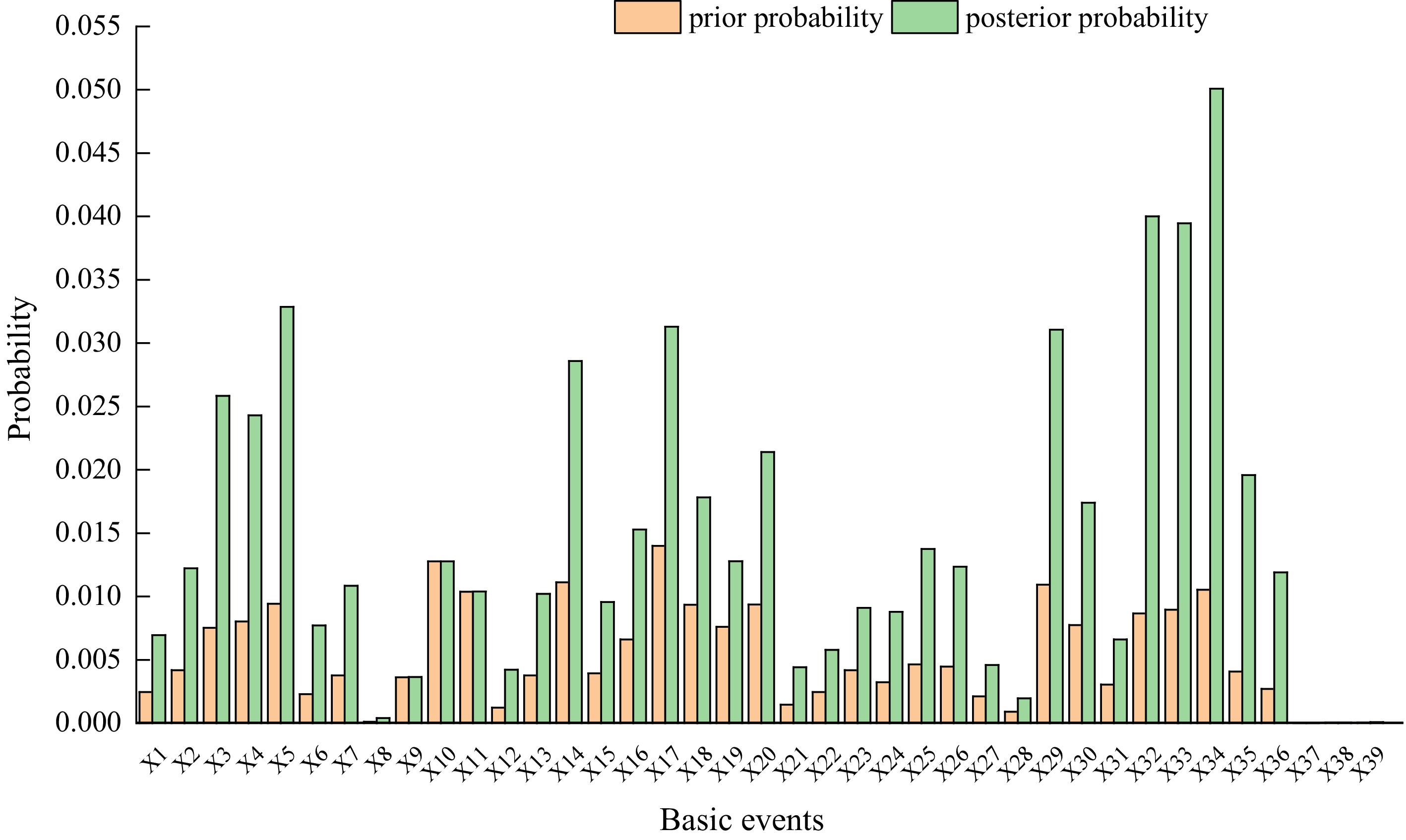
Figure 3.
Comparison of the prior and posterior probabilities of basic events.
Sensitivity analysis
-
Sensitivity analysis is employed to identify the basic events that significantly influence the result. The Ratio of Variation (RoV) is used to calculate the effect of the underlying event on the probability of the outcome failure. A higher RoV value indicates that the corresponding basic event has a greater impact on the top event. The RoV value is calculated as follows:
$ RoV({x_i}) = \dfrac{{P({x_i}) - Q({x_i})}}{{Q({x_i})}} $ (15) where, RoV(xi) is the rate of change. P(xi) is the posterior probability of xi, and Q(xi) is the prior probability of xi.
Based on the sensitivity analysis results calculated using the formula, the RoV values for the basic events are given in Fig. 4. The analysis indicates that events X8 (third-party destruction), X32 (gasket failure), X33 (seal failure), X34 (flange scouring and wear), X35 (valve scouring and wear), and X36 (deterioration of accessories) have higher RoV values. This means that even small changes in the probabilities of these events can significantly impact the probability of the top event. Therefore, special attention should be paid to the aging, failure, and wear of accessories during routine maintenance.
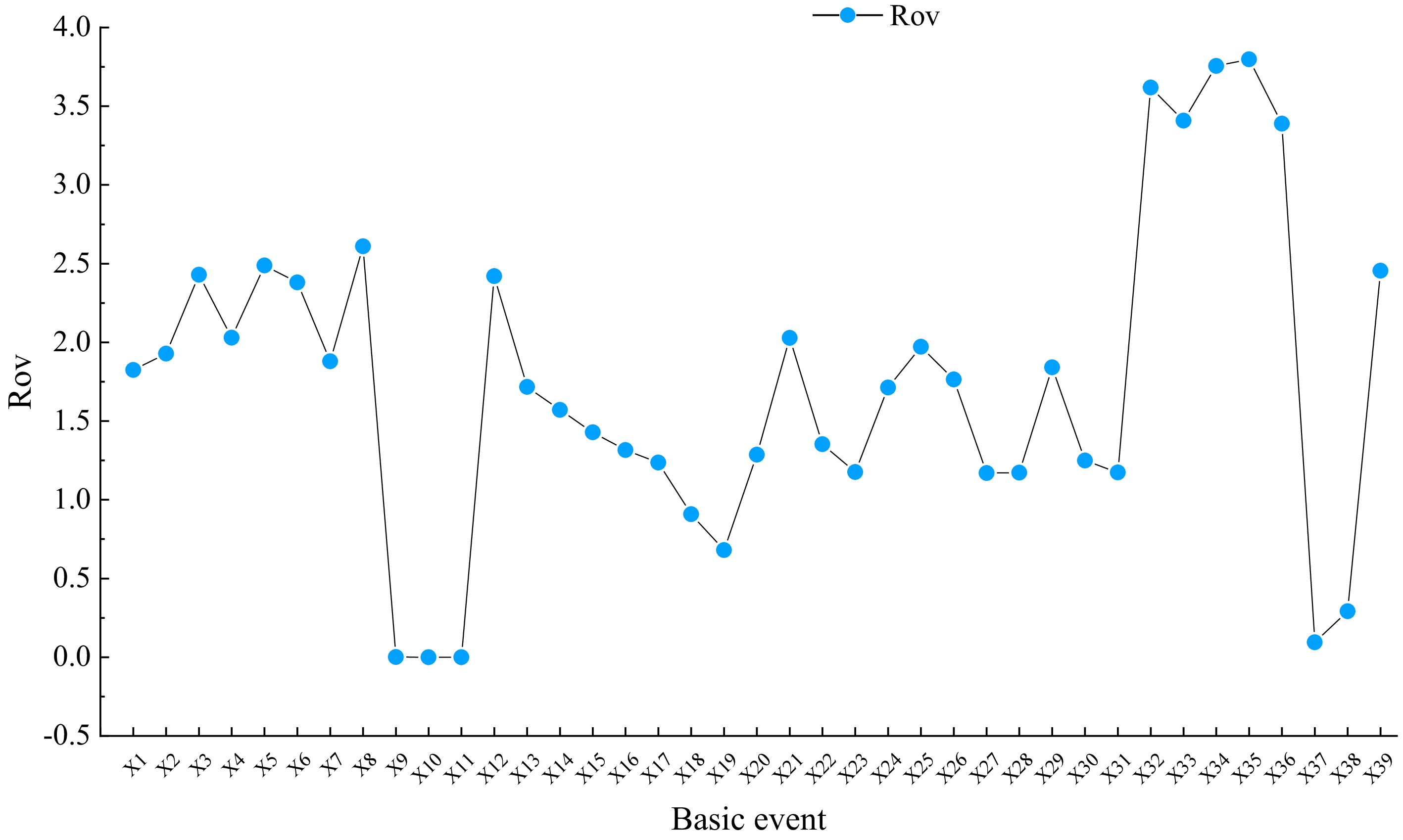
Figure 4.
Basic event RoV value.
Maximum causal chain analysis
-
Bayesian maximum causal chain analysis is an inference method based on Bayesian networks, primarily used to identify the key causal chain through which a top event occurs, allowing for the precise identification of the hazard's source. This method performs an influence strength analysis, where the thickness of the connecting arcs in the model visually represents the strength of influence relationship between nodes.
Using the Bayesian network model of syngas leakage and the 'strength of influence' function in GeNIe software, the maximum causal chains leading to syngas pipeline leakage can be effectively identified.
Figure 5 presents the causal chain analysis for syngas pipeline leakage and obtains the strength of the causal relationships by the thickness of the connecting lines. Starting from T, the thickest connecting lines are identified step-by-step, among the three parent nodes M1, M2, M3 of T, M2 is thickest; Among the two parent nodes M6, M7 of M2, M6 is thickest; Among the four parent nodes M8, M9, M10, M11 of M6, M10 is thickest; Among the four parent nodes M12, M13, M14, M15 of M10, M14 is thickest; Finally, among the two parent nodes X24, X25 of M14, X25 is thickest. Therefore, the maximum causal chain leading to syngas pipeline leakage is: (X25 → M14 → M10 → M6 → M2 → T), i.e., deformation of the cooling ring → burn-through of drop tube → pipe overheating → syngas pipeline leakage → equipment factors → gasifier syngas pipeline leakage. Additionally, other critical chains leading to the syngas pipeline leakage can also be identified. For instance, if the basic event X26 chain is thicker, this indicates that the X26 internal structure is the source of the most approximate causal chain for the parent node M15 overheating of the pipe. This approach enables the identification of key risk factors and provides data support for further risk prevention, control, and management.
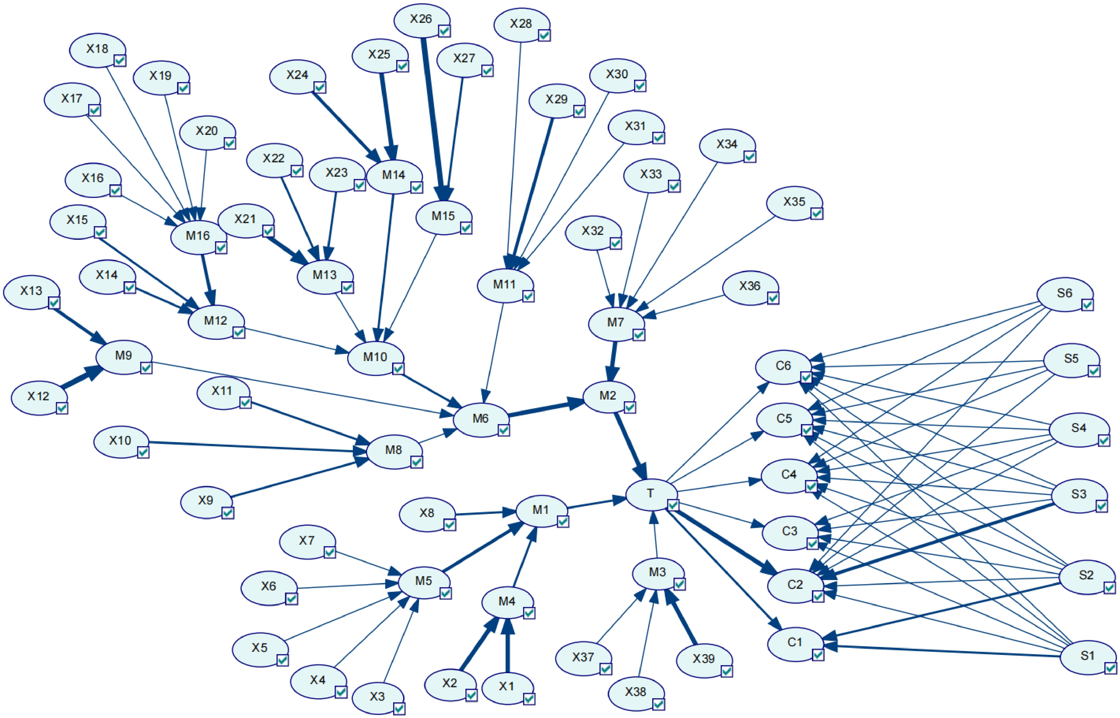
Figure 5.
Causal chain analysis.
Dynamic probability analysis
-
The selected dynamic basic events are X9, X10, X11, X12, X13, X34, X35, and X36, and use two-parameter Weibull distribution to realize dynamic node probabilities transfer over neighboring time segments in the DBN. The time slice is set to 24, representing 24 months, and click update. Through the transmission of transfer probability in DBN, the dynamic update of the probability of syngas pipeline leakage and consequence accidents over time can be realized, and the change rule of probability over time can be predicted.
Figure 6 presents the temporal evolution of the probabilities for the consequence events C3 (jet fire), C4 (vapor cloud explosion), C5 (flash fire), and C6 (poisoning asphyxiation). The probability of each consequence event gradually increases over time. At the same point in time, the occurrence probability of every consequential event ranks as follows: jet fire > flash fire > poisoning asphyxiation > vapor cloud explosion. Jet fire starts with the highest initial probability, and its probability grows most significantly when safety barriers fail. This is mainly because the syngas pipeline operates at a high pressure of up to 4 MPa, causing high-velocity gas release upon leakage, which readily triggers a jet fire when an ignition source is present. Although the probability of a vapor cloud explosion occurring is relatively low, once it does, the danger posed is the greatest and may result in serious casualties and equipment damage. In practice, we still need to maintain a high degree of vigilance on it. In practical operations, once a leak is detected, rapid emergency response is essential to mitigate the impact and avoid catastrophic consequences.
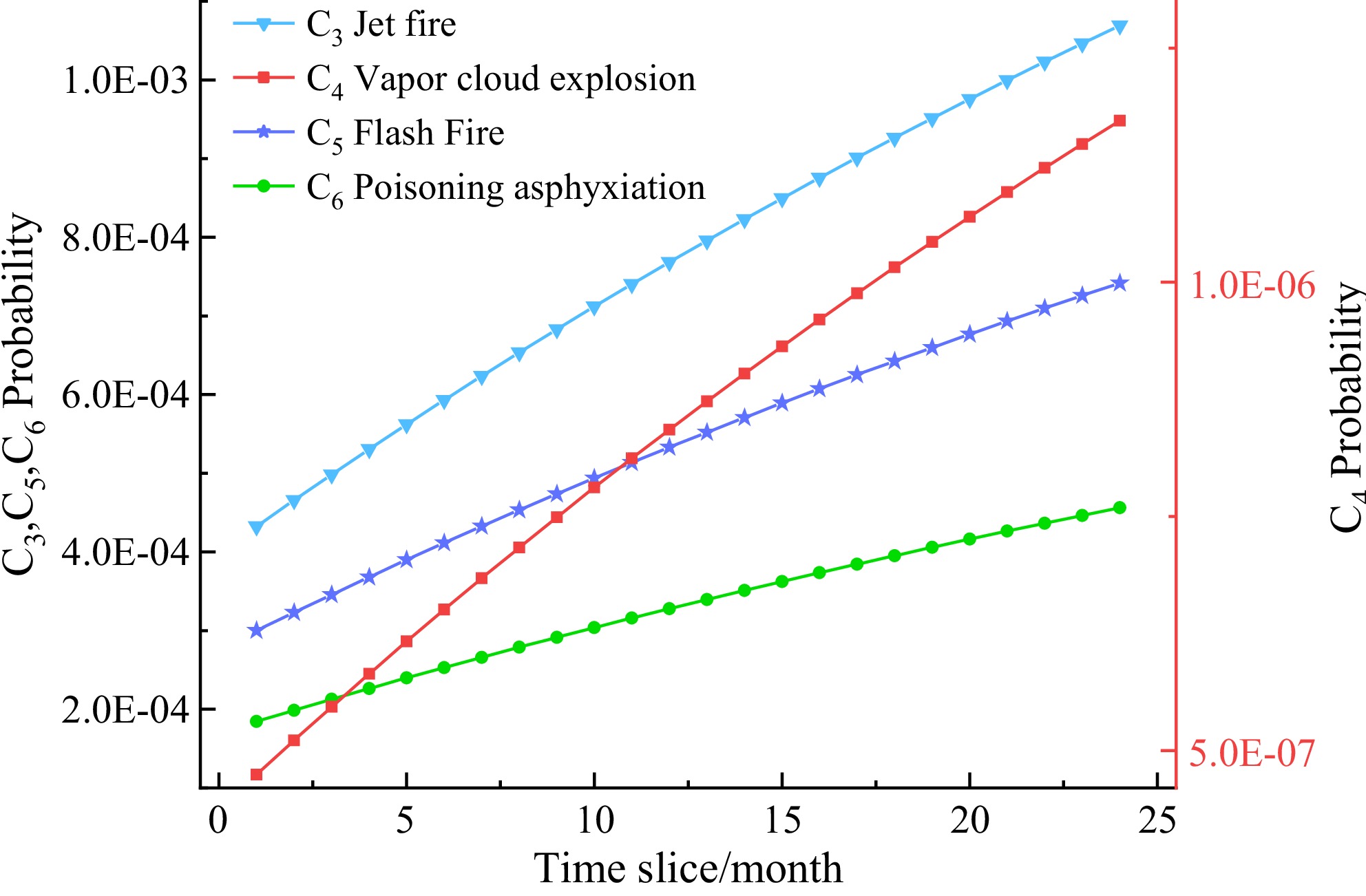
Figure 6.
Changes in probability of consequences of syngas leaks.
Figure 7 illustrates the trend curve of syngas pipeline leakage probability over time. The initial leakage probability is 0.118055, and this value is consistent with the static BN analysis results, thereby verifying the reliability of the method. The leakage probability gradually increases over time, reaching 0.2918 after 24 time slices, indicating a rising risk during the accumulation process. The rate of growth slows down as time increases.
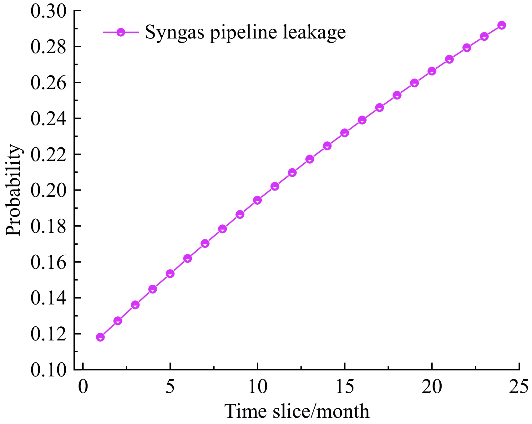
Figure 7.
Change in probability of syngas leakage.
Therefore, in the actual process, the real-time monitoring of key nodes should be enhanced, and timely maintenance and inspection should be conducted to ensure process safety, minimize leakage risk, and reduce potential environmental pollution and direct economic losses.
-
(1) The paper focused on the leakage risk of syngas pipelines in coal gasification. A risk identification model was developed using BT analysis. The BT model was converted to the DBN model through a mapping algorithm. Fuzzy set theory, and improved SAM method was applied to process expert judgments and derive the priori probabilities.
(2) Key hazard events were identified including X3, X4, X5, X14, X17, X29, X32, X33, X34. Their high posterior probabilities indicate that these are the primary sources of risk contributing to syngas pipeline leakage.
(3) Sensitivity analysis revealed several basic events, X8, X32, X33, X34, X35, X36, with high RoV values, indicating their strong influence on leakage risk. Even small changes in their probabilities can significantly increase the risk of pipeline leakage. Therefore, these highly sensitive factors should be given priority in safety management. The maximum causal chain identified was X25 → M14 → M10 → M6 → M2 → T.
(4) The predictive inference function of DBN can be used to obtain the probability of syngas leakage and the characteristics of the consequence events over time. The leakage probability increased from an initial 0.1181 to 0.2918 over 24 time slices. The risk of leakage increased gradually during the cumulative process of time, but its growth rate was gradually leveling off. The probability ranking of consequential events was jet fire > flash fire > poisoning asphyxiation > vapor cloud explosion.
(5) In the paper, a DBN risk analysis method for the leakage of a coal gasification syngas pipeline is proposed. Realized dynamic risk assessment of syngas pipeline leakage and could provide a reference for routine maintenance, risk warning, and emergency response planning.
The authors are grateful to the financial support of The Key Research and Development Program (High and New Technology) of Ningxia Hui Autonomous Region (2022BEE02001).
-
The authors confirm contribution to the paper as follows: study conception and design: Liu Y, Hua M; data collection, processing, and paper writing: Liu Y; review of the results, revision, and approvement of the final version of the manuscript: Hua M, Pan X. All authors reviewed the results and approved the final version of the manuscript.
-
The datasets generated during and/or analyzed during the current study are available from the corresponding author on reasonable request.
-
The authors declare that they have no conflict of interest.
- Copyright: © 2025 by the author(s). Published by Maximum Academic Press on behalf of Nanjing Tech University. This article is an open access article distributed under Creative Commons Attribution License (CC BY 4.0), visit https://creativecommons.org/licenses/by/4.0/.
-
About this article
Cite this article
Liu Y, Hua M, Pan X. 2025. Risk assessment of syngas pipeline leakage based on a Dynamic Bayesian Network. Emergency Management Science and Technology 5: e013 doi: 10.48130/emst-0025-0011 

Risk assessment of syngas pipeline leakage based on a Dynamic Bayesian Network
- Received: 23 March 2025
- Revised: 13 May 2025
- Accepted: 05 June 2025
- Published online: 07 July 2025
Abstract: The syngas pipeline serves as the primary carrier for syngas exported from the coal gasification furnace, is vulnerable to corrosion and erosion from the transported medium, and is prone to leakage due to long-term high-pressure operation. Moreover, due to its compositional characteristics, syngas pose flammability, explosive, and toxicity risks, which can potentially lead to severe accidents if a leak occurs. Therefore, it is essential to conduct a risk assessment of syngas pipeline leakage. This study proposes a risk assessment approach for syngas pipeline leakage in coal gasification using Dynamic Bayesian Network (DBN). First, the risk identification model is built using Bow-Tie (BT) analysis and then mapped into DBN using a mapping algorithm. Expert evaluation, improved similarity aggregation methods, and fuzzy set theory are employed to quantify prior probabilities. To address the uncertainty of the DBN model, a Leak Noisy-or gate model is introduced. Time series are added to predict the dynamic probabilities. Nine key hazard events, six highly sensitive factors, and the maximum causal chain are identified, and predict the dynamic probability of syngas pipeline leakage and potential consequences. This study provides a theoretical basis for routine maintenance and risk assessment of syngas pipelines.
-
Key words:
- Dynamic Bayesian Network /
- Syngas pipeline /
- Risk assessment