Genomic mating strategy for papilla number in Apostichopus japonicus

Sea cucumber Apostichopus japonicus is one of the most economically important aquaculture species in the Western Pacific region, prized for its nutritional and medicinal value^[1]. Since sea cucumbers with more papillae fetch higher market prices, the number of papillae is regarded as a primary selection goal in breeding research^[2]. However, problems such as overfishing and inbreeding depression resulting from the rapid expansion of aquaculture have led to a reduction in effective population size and a significant decline in sea cucumber germplasm resources^[3]. The lag in the collection and protection of sea cucumber germplasm resources has made the problem increasingly prominent, which has diminished their ability to resist diseases and environmental stress, often leading to large-scale mortalities during aquaculture, resulting in significant economic losses, and ultimately, seriously affecting the healthy development of the sea cucumber aquaculture industry. Therefore, there is an urgent need for a breeding method that selects individuals with desirable traits to improve economic benefits and maintain the level of genetic diversity within the population, ensuring the sustainability of A. japonicus breeding industry.

Genomic selection (GS), a breeding technique that utilizes molecular markers covering the whole genome, has emerged with the rapid development and widespread application of high-throughput sequencing and genotyping technologies^[4]. Compared to pedigree-based best linear unbiased prediction (BLUP) and marker-assisted selection (MAS), GS uses genome-wide markers for breeding value estimation, which improves the accuracy of estimating breeding values. Additionally, GS enables early genotyping of individuals, significantly shortening the generation interval and improving breeding efficiency^[5]. However, similar to other breeding methods based on estimated breeding values, GS still involves truncation selection, where individuals below a certain selection threshold are eliminated to form the next generation population^[6]. Jannink^[7] suggested that GS could reduce breeding cycle time and greatly increase early selection gain, but also resulted in the loss of favorable quantitative trait locus (QTL) alleles, leading to a loss of genetic variance and eventual reduction in GS accuracy. Wientjes et al.^[8] simulated long-term effects of GS and found that the accuracy of selection, the rate of genetic gain, the amount of additive genetic and genetic variation, and the number of segregating causal loci decreased after long-term selection. Consequently, while GS can significantly increase genetic gains in the short term, it may lead to the purging of alleles and a reduction in genetic variation within the breeding population, ultimately resulting in inbreeding depression. This limitation hampers the long-term gains in the selected traits and jeopardizes the future reproductive potential of other traits^[7].

Different from randomly mating high breeding value individuals, optimized mating methods based on pedigree relationships preserve the contribution potential of each individual as a parent, allowing for a balance between obtaining genetic gains and controlling the average degree of inbreeding and probability of shared ancestors^[9]. This approach aims to maintain sustainable long-term genetic gains and enables the selection of appropriate mating schemes based on different breeding objectives. With the widespread application of genomic molecular markers, such as single-nucleotide polymorphisms (SNPs), genomic mating (GM), a method that uses genomic information to optimize parental mating combinations, has emerged^[10].

To address the predicaments of GS in long-term selection, the key to GM is to maximize genetic gain while simultaneously controlling the kinship among breeding individuals. The optimum contribution selection (OCS) algorithm was used to solve this problem^[9]. This method controls the genetic contribution of each candidate parent, thereby limiting the accumulation of coancestry among offspring and promoting sustainable long-term genetic gain. The theory of genetic contributions posits that the maximum rate of genetic gain is achieved when an optimal threshold linear relationship exists between the Mendelian sampling of ancestors and their genetic contributions to the descendants, under restricted parental relationships. This theory underpins the OCS algorithm, which has been shown to effectively balance genetic gain and genetic diversity in breeding programs^[11]. With the advent of genome-wide SNPs, tracing of chromosome segments has become feasible, allowing for more accurate estimation of relationships among candidate parents. Genomic optimal contribution selection (GOCS) can achieve a closer approximation to the exact threshold linear relationship by utilizing genomic information, thereby enhancing the accuracy of Mendelian sampling evaluation^[12,13]. At present, GM has been studied in several important livestock species, such as dairy cattle, but there are fewer reports in aquaculture breeding.

In this study, we utilized real genotype and phenotype data from sea cucumber samples collected from eight different geographic regions to simulate breeding for the complex trait of papilla number. To assess the long-term applicability of GM strategies in aquaculture breeding, we conducted simulations comparing average genetic gains and inbreeding coefficients across generations under two GM schemes and three GS schemes. The results demonstrated that, in long-term breeding, GM not only achieved higher genetic gains compared to GS but also effectively controlled the inbreeding coefficient. These findings provide theoretical support for the effective selection and breeding of superior A. japonicus strains.

A total of 215 sea cucumbers were collected from seven different aquaculture geographic locations, including Bashao Island (BSD), Russia (ELS), Huanglongwei (HLW), Lvshun (LS), Pingdao (PD), Qixiakou in Shandong (SD), and Xixiaomo (XXM), and one Sino-Russian hybrid aquaculture population (SYNo). The commercially important trait, papilla number, was recorded according to the method of Chang et al.^[2]. The number of papillae was counted and directly recorded by an investigator.

The papilla tissues were quickly frozen in liquid nitrogen and then stored at −80 °C for DNA extraction. First, DNA was extracted using the DNeasy Blood & Tissue Kit (Qiagen, Shanghai, China), and quantification analysis was performed using NanoDrop-2000 (Thermo Scientific). Then, the NEBNext Ultra DNA library Prep Kit (New England BioLabs, United Kingdom) was used for library preparation. Finally, libraries were sequenced using the Illumina HiSeq2500 platform in PE150bp mode, with a sequencing depth of 10× for each sample.

Raw sequence reads were subjected to stringent quality control, including base quality filtering and adapter trimming, using Trimmomatic version 0.38^[14]. Low-quality reads with average Phred-equivalent quality scores < 20, or containing more than five consecutive bases or ambiguous nucleotides (denoted as Ns) were discarded in further analysis. The obtained high-quality sequencing data were aligned to the A. japonicus reference genome^[15] using BWA version 0.7.17-r1188^[16] to generate BAM files. Picard version 2.27.5 (https://broadinstitute.github.io/picard/) was used to sort the BAM files, identify and remove duplicate reads, and assign all the reads in a file to a single new read group. Variant calling was performed using Freebayes version 1.3.6^[17] after indexing with SAMtools version 1.17^[18], after which small insertions and deletions (INDELs) exclusion and SNP filtering were accomplished using VCFtools version 0.1.16^[19]. Then, the retained SNPs were further filtered using VCFtools version 0.1.16. SNPs with >2 alleles, minor allele frequency (MAF) < 0.05, and calling rate < 0.9 were excluded from the high-quality SNP set. Subsets of 1,500, 1,000, 500, 250, 100, 75, 50, 25, 15, and 10 K SNPs were randomly screened from the high-quality SNP set (three replicates were done for each density subset) to calculate the genomic prediction accuracies, and thus determine the number of SNP loci to be used in this study.

Initial population genetic structure

A genomic kinship matrix of 215 sea cucumbers based on high-quality SNP data was inferred using TASSEL version 5.2.94^[20], and principal component analysis (PCA) was executed with PLINK version 1.90b6.18^[21] after performing linkage disequilibrium (LD) pruning. The genetic composition of the samples was inferred utilizing ADMIXTURE version 1.3.0^[22] with K values ranging from 1 to 8, and the optimal K value was determined based on the lowest cross-validation error. A population stratification diagram, employing the optimal K value, was generated with TBtools-II version 2.119^[23]. Additionally, PopLDdecay version 3.42^[24] was used to assess the pairwise LD and R-squared correlation coefficients (r²) between alleles. The LD decay plot was created utilizing a Perl script integrated within the software.

Breeding strategy

A 230 K SNP dataset and 215 initial individuals were employed to implement five breeding strategies, with additive and dominant effects estimated for every locus. Candidate selection for progeny generation was conducted by GS through maximising genomic estimated breeding values (GEBVs), and by GM through maximising genetic gain and minimising kinship, respectively (Fig. 1). All strategies were implemented in R and ran on a Linux machine with an Intel Core i5-3230M CPU processor @2.60GHz with 4 GB of RAM memory. The genetic structure of the 20^th generation of the simulated population was inferred using ADMIXTURE version 1.3.0^[22].

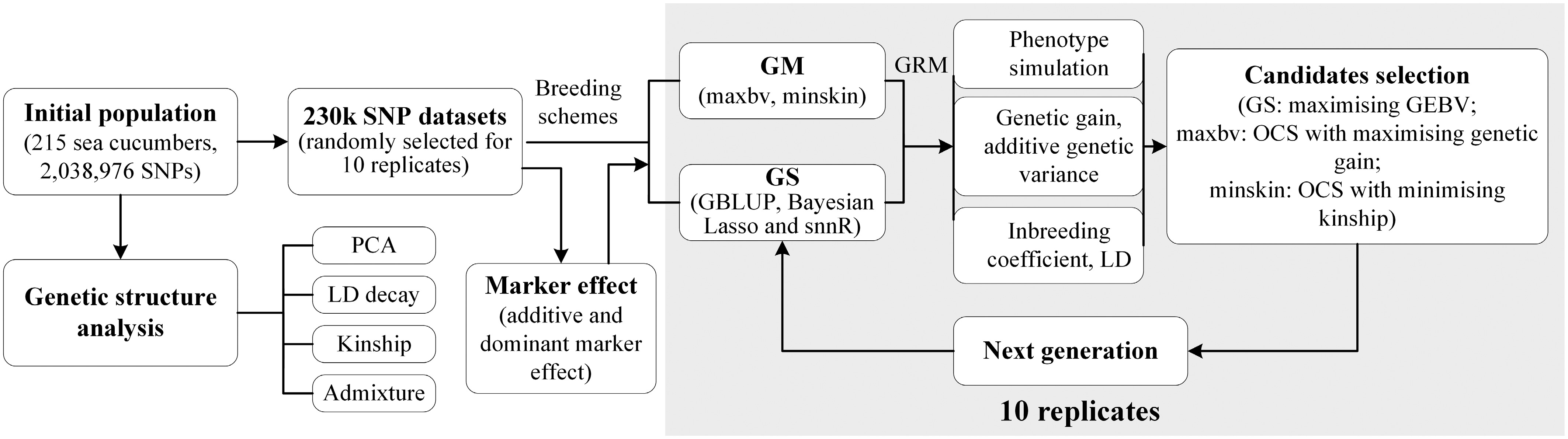
Figure 1. 

Construction process of genomic selection (GS) and genomic mating (GM) for breeding simulation.

Genomic selection

Two linear genomic prediction methods, genomic best linear unbiased prediction (GBLUP) and Bayesian least absolute shrinkage and selection operator (Bayesian Lasso), and one nonlinear neural-network method, snnR, were used in the breeding simulation. For each breeding scheme, simulations were conducted ten times, and PC1 and PC2 were used as fixed effects. Additive effects were used for GEBV calculation, and both additive and dominance effects were included to generate the genotypic value. According to the estimation of breeding values for offspring individuals, in each generation, the top 50 individuals with the highest GEBVs were selected for random mating to produce the next generation.

GBLUP, implemented using the 'synbreed' R-package, assumes that all markers have equal variance and small effects, and estimates additive genetic effects based on the genomic relationship matrix (GRM), which was calculated using the kin() function from the 'synbreed' R-package^[25]. The model equation is as follows^[26]：

where, y denotes the phenotype vector; X is a fixed effects matrix associated with each individual and b is a vector of fixed effects; Z represents the matrix associated with genetic values; g denotes the vector of additive genetic values for an individual and $ e\sim N\left(0,{\sigma }^{2}\right) $, denotes the residual vector. Moreover, G represents the genomic relationship matrix, and $ \sigma _{g}^{2} $ denotes the genetic variance within this model.

Bayesian Lasso model, implemented using the 'synbreed' R-package, includes only a subset of explanatory variables, with other variables set to zero^[27]. This is consistent with the assumption proposed by Hayes & Goddard^[28] that only a small number of chromosome segments contain real QTLs. The Markov chain length was 600,000, with the first 30,000 discarded as a burn-in period. The specific model is as follows:

where, y is the n*1-dimensional phenotype vector, β is the fixed-effects vector, e is the n*1-dimensional residual, W is the n*p-dimensional marker matrix, and m is the p-dimensional vector of SNP effect values.

The snnR model is a sparse neural network breeding algorithm proposed by Wang et al.^[29]. The method constructs a sparse deep neural network by reasonably reducing internal connections through L1 regularisation applied to every single hidden layer^[30]. The maximum number of iterations was determined to be ten, based on the volume of the input data, with early stopping employed to prevent overfitting. Following the approach of Wang et al.^[29], the neural network was configured with three hidden layers, each comprising five neurons, and utilized the activation functions and L1-norm penalty that are default in the 'snnR' R-package.

Single hidden layer neural networks:

The sparse structure is obtained by constraining the extremes of this model through the L1-norm penalty:

where, $ {y}_{i} $ is the trait measured on individual i, µ is an intercept, $ {x}_{ij} $ (i = 1, …, n denoting the individual and j = 1, …, p denoting the marker) is the genomic covariates, $ \beta _{j}^{\left[k\right]} $ is a vector of input weights, $ {b}_{k} $ (k = 1, …, S denoting a neuron) is an intercept, called 'bias' in NNs, $ {g}_{k}\left(.\right) $ is an activation function producing the output of the single hidden neuron, $ {W}_{k} $ denote weights in the output layer, and $ {\varepsilon }_{i}\sim NIID\left(0,\sigma _{e}^{2}\right) $, where $ \sigma _{e}^{2} $ is the residual variance. $ \hat{\mathcal{L}}\left({W}_{k},{b}_{k},\beta _{j}^{\left[k\right]}\right) $ is the approximate square error, $ {\lambda }_{k,j} $ and $ {\lambda }_{k} $ are Lagrange multipliers that determine the amount of sparsity in $ \beta _{j}^{\left[k\right]} $, $ {W}_{k} $ and $ {b}_{k} $.

Genomic mating

'optiSel' R-package^[31] was used for OCS calculations. Estimation of kinship $ {f}_{ij} $ was conducted using the runs of homozygosity (ROH)-based method^[32]. The method of de Cara et al.^[33] was used to define kinship as:

where, $ {L}_{k}({a}_{i},\;{b}_{j}) $ refers to the length of the k^th shared IBD segment measured through the homologous chromosome a of individual i and the homologous chromosome b of individual j. L is the total length of the genome. In addition, we set the total genetic contribution of all males to 1/2, equal to that of females.

When the goal of mating is to maximise genetic gain, as the inbreeding coefficient of an individual is equal to the kinship of its parents, the breeding goal can be transformed to restrict:

where, $ {n}_{ij} $ is the offspring of individual i paired with individual j, M contains all candidate male parents, F contains all candidate female parents, and N is the total number of offspring and $ {f}_{ij} $ is the kinship matrix. The upper limit of kinship was set in this study as:

where, Kin is the average population kinship, $ Kin=Z{Z}^{'}/2\sum{p}_{i}(1-{p}_{i}) $, where $ Z=W-P $, $ W $ is the marker matrix, $ P $ contains the allele frequencies multiplied by 2, $ {p}_{i} $ is the allele frequency of marker $ i $, and the sum is over all loci. Ne is set to 100 for the effective population size^[12,31], and L is the generation interval based on the contribution of the individuals to the current population^[31]. Subject to this kinship constraint, by maximising the Lagrangian objective function, the optimal c-vector, i.e., parental contribution, matrix was obtained.

When the goal of mating is to minimise the kinship coefficient, the mating problem can be expressed by the following equation.

where, r is the mean genetic correlation, G is the genomic relationship matrix, X is the centralized genotype matrix, c is the vector of proportional genetic contributions of individuals to the next generation, b is the vector of GEBVs for the candidate individuals, and $ \rho $ is the average GEBV of the next generation. When the objective is to minimize mean kinship, the threshold for the constraint is set to the average breeding value of the candidate individuals^[31].

Similarly, PC1 and PC2 were used as fixed effects in GM strategies. Different from GS, GM did not fix the number of candidate parents, but automatically calculated the contribution value of each individual according to the optimisation objective and constraints, and then obtained the optimal offspring individuals based on the contribution value prediction. The number of offspring and the sex ratio in GM were the same as those in GS. Each programme simulated 20 generations of breeding, with ten generations defined as short-term selection and 20 generations as long-term selection^[34]. Simulations were repeated ten times for all generations of each breeding strategy.

Simulated scenarios

Simulation theory and genomic settings

The result of the rapid decay of LD in the initial population indicated low correlation between loci. All loci were assumed to be physically unlinked, and no epistatic interactions were simulated. Gamete splitting was performed on the parents to simulate meiosis. The number of QTLs was identical to the number of SNP loci, and they were uniformly distributed across the chromosomes. And the SNP-based heritability of papilla number was estimated to be 0.7, indicating a high heritability. Estimate the environmental variance based on the genetic variance and heritability. The 'hypred' R-package^[35] was used to simulate the meiosis process, with a mutation rate of 2.5 × 10⁻⁵ for both SNP loci and QTL loci and a recombination rate of 1 cM/Mb.

Simulation of offspring phenotype

Phenotypic simulations for the traits of papilla number in sea cucumbers fit the following model:

where, $ {y}_{i} $ is the phenotype of individual i. $ {G}_{i} $ and $ {E}_{i} $ are the genotype value and the environmental effect for that individual, respectively. Environmental effects are taken from a normal distribution $ N(0,\;\sigma _{e}^{2}=sd\left(bv\right)) $. $ {G}_{i} $ values consist of additive and dominant effects, a and d, which are set to be constant between generations for each QTL according to the method of Xiang et al.^[36], with no variation over time or environmental conditions. The phenotype of each individual was determined by its genotypic value and environmental effects, without repeated measurements or maternal effects.

Genetic gain and genetic parameter of offspring

Genetic gain and additive genetic variance

Genetic gain is defined as the average genotypic value (true genetic performance) of the current generation, taking into account additive and dominance effects^[35].

The additive genetic variance for each generation was calculated using the genome-based restricted maximum likelihood (GREML) linear mixed model of the GCTA version 1.94.1^[37] as follows:

and the variance is:

where, y is a vector of n*1 phenotypes, n is the sample size, $ \beta $ is the coefficients of the fixed effects covariates, X is the incidence matrices for fixed effects, A denotes the GRM, and G is an n*1 vector representing the genetic effects for each individual, obeying g~N(0, $ A\sigma _{g}^{2} $), and e denotes the random error.

Inbreeding and LD

The inbreeding coefficient was calculated using the R package 'optiSel', defined as the probability that a paternal and a maternal allele sampled at a random locus both fall within a run of homozygosity (ROH)^[33]. LD calculation was achieved by GCTA version 1.94.1^[37], setting up windows with a length of 10 MB. The r² between all SNPs in each window was counted, and r² less than 0.01 was filtered^[34].

Supplementary Table S1 summarized the phenotypic data of papilla number for a total of 215 sea cucumbers from eight different geographical locations, with mean values (Mean ± SD) of 47.90 ± 9.45 (BSD), 56.67 ± 10.72 (ELS), 34.63 ± 4.79 (HLW), 34.23 ± 5.14 (LS), 44.47 ± 6.06 (PD), 40.80 ± 4.40 (SD), 58.40 ± 6.88 (SYNo), and 50.50 ± 9.18 (XXM), respectively (Supplementary Table S1 and Fig. 2a).

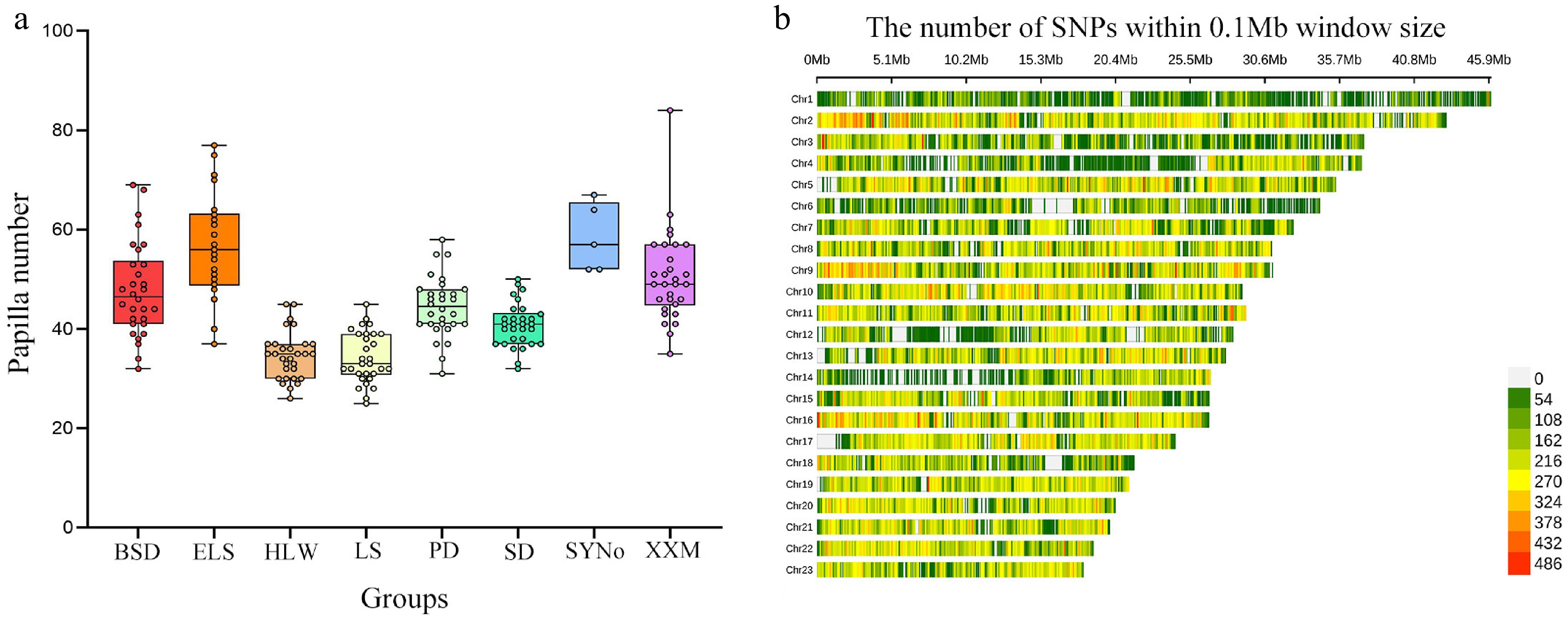
Figure 2. 

Phenotypic and genotypic data for the initial population. (a) Statistics for papilla number of 215 sea cucumbers from eight different geographical locations. (b) SNP density distribution plot.

Whole-genome sequencing (WGS) was conducted for 215 sea cucumbers, resulting in roughly 1.6 TB of clean reads post-quality filtration. Following rigorous quality control, 2,038,976 high-quality SNPs were confirmed for further analysis, and the chromosome-specific SNP count varied (Fig. 2b). By calculating genomic prediction accuracies across subpanels with different densities and considering the requirements of the current script for the dataset, 230 K SNPs were ultimately selected as the input genotype data (Supplementary Fig. S1).

Genetic structure and parameter analysis of the initial population

Based on the principal component analysis results (Fig. 3a), clear genetic stratification was observed between the 30 individuals collected from Russia and the local populations from Shandong and Liaoning in China, according to the first two principal components, PC1 (19.16%) and PC2 (11.22%). Notably, five hybrid individuals, shown in purple in the figure, were positioned between the Russian and Chinese samples, suggesting they may have mixed genetic backgrounds. The fast rate of LD decay suggested high genetic diversity in the initial population (Fig. 3b). The kinship matrix constructed using the Centered_IBS method of the TASSEL software is shown in Fig. 3c. Most of the kinship coefficients between pairs of individuals were below 0.1, suggesting a weak genetic relationship within 215 individuals. The population structure analysis (Fig. 3d, e) also indicated that K = 2 yielded the lowest CV value of 0.65580. At K = 2, the Russian and Chinese populations represented the two major genetic components, while the hybrid individuals displayed mixed ancestry, reflecting their intermediate genetic composition. These results indicated that the initial population can be divided into two subgroups: the Russian population and the Chinese population, with evidence of admixture in a few individuals.

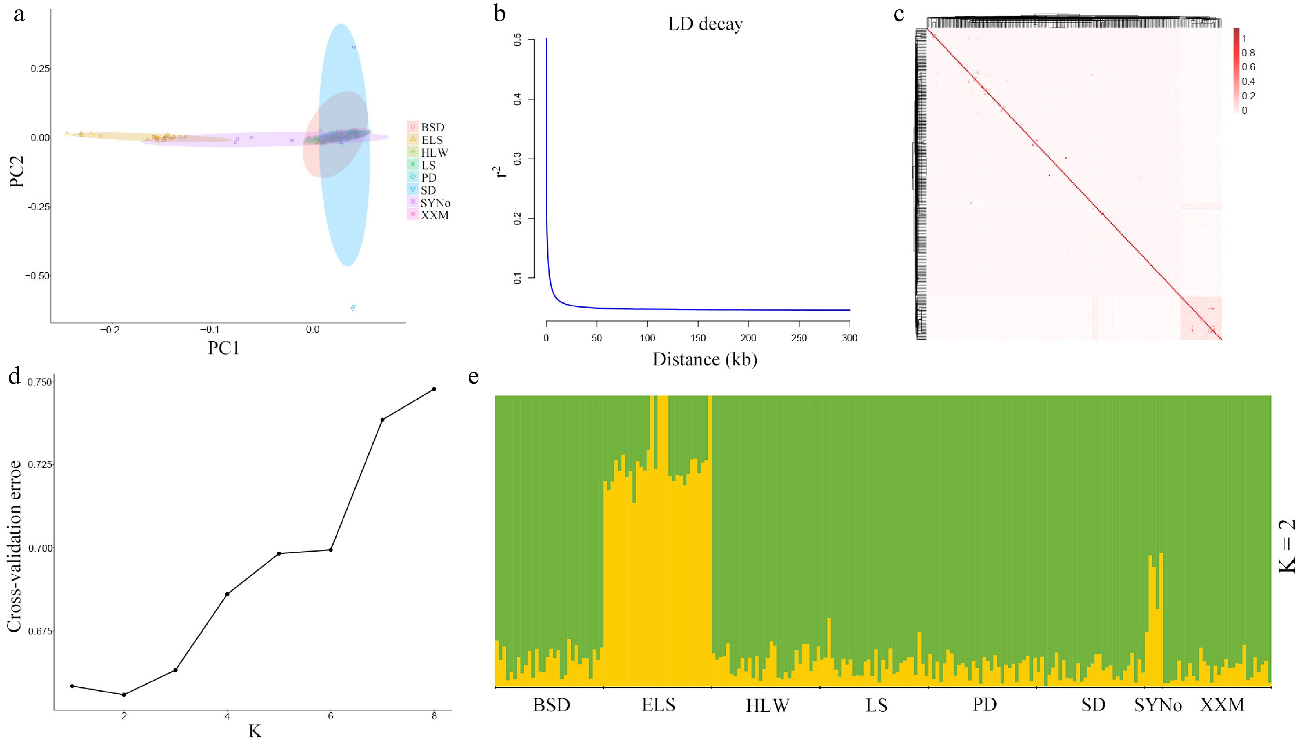
Figure 3. 

Population genetic analysis of 215 sea cucumbers of the initial population. (a) Principle component analysis (PCA) plots. (b) LD decay plot. (c) Heatmap plot of kinship. (d), (e) Population genetic structure.

Phenotype simulation

The distributions of additive effects and dominance effects for the selected 230 K SNPs were shown in Supplementary Fig. S2. Both distributions followed a normal distribution, indicating that they meet the assumptions of the analysis.

To assess the credibility of the simulated phenotype, ten sets of randomly selected genotype data were selected to simulate the phenotypes for the initial population. The QQ plot shows that the simulated phenotype closely follows a normal distribution (Supplementary Fig. S3).

Genetic parameters of genomic selection and genomic mating

Genetic gain, additive genetic variance, inbreeding coefficient, and LD were compared across five breeding strategies over 20 generations.

Genetic gain and additive genetic variance

After a comprehensive comparison of the five strategies in the 20 generations of selection, the results indicated that:

In terms of genetic gain, Fig. 4a showed that the genetic gain of 'maxbv' was 30.41%, 14.26%, 22.45%, and 2.71% higher than GBLUP, Bayesian Lasso, snnR, and 'minskin' after short-term selection, respectively; while the genetic gain of 'maxbv' was 68.99%, 32.28%, 53.07%, and 2.75% higher than GBLUP, Bayesian Lasso, snnR, and 'minskin' after long-term selection, respectively (all values represent relative percentage differences relative to the results of other groups). The results for all generations indicated that the 'maxbv' strategy consistently had the highest genetic gain, while 'minskin' had a slightly lower genetic gain. The genetic gain of the three breeding strategies for GS was consistently lower than that of the two GM strategies. As the generation of simulations increased, the genetic gain of all breeding strategies first underwent an upward trend and then fell back, with the GBLUP showing the fastest decline in genetic gain.

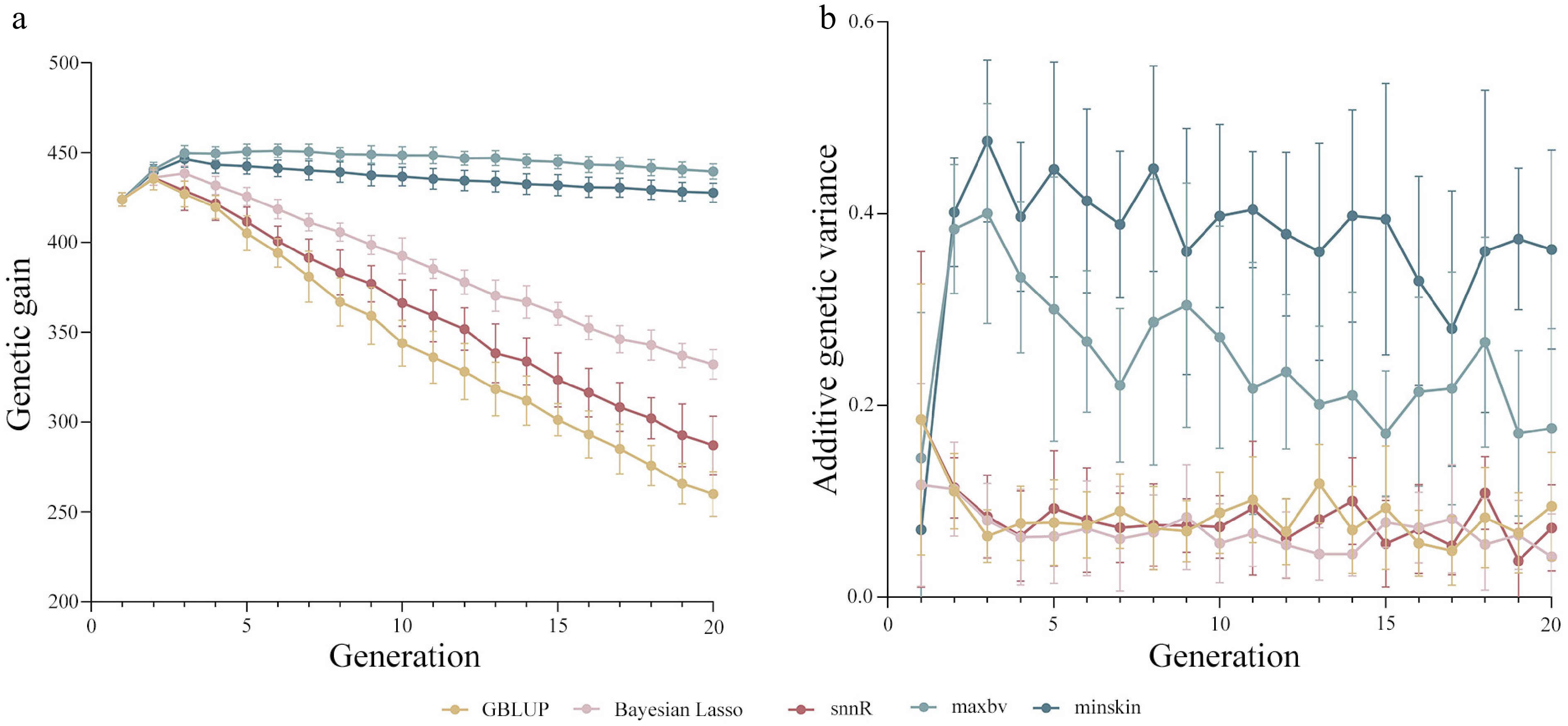
Figure 4. 

(a) Genetic gain, and (b) additive genetic variance of genomic mating (GM) and genomic selection (GS) schemes on papilla number in all generations.

In terms of additive genetic variance, Fig. 4b demonstrated that all GS strategies followed a decreasing tendency, and both GM strategies presented an upward then downward tendency. The additive genetic variance for GM strategies was consistently higher than that of the GS schemes from the second generation onwards. By generation 20, compared to 'maxbv', the additive genetic variance of GBLUP, Bayesian Lasso, and snnR was reduced by 46.05%, 76.05%, and 58.95%, respectively; in comparison to 'minskin', the additive genetic variance of GBLUP, Bayesian Lasso, snnR, and 'maxbv' decreased by 73.81%, 88.37%, 80.07%, and 51.45%, respectively.

Inbreeding and LD

In terms of inbreeding level (Fig. 5a), the 'minskin' strategy demonstrated the lowest level of inbreeding throughout, while the other GM strategy 'maxbv' had a slightly higher inbreeding level than 'minskin' without exceeding 0.05. In terms of short-term selection, the inbreeding coefficients of 'minskin' were 95.57%, 92.98%, 94.67%, and 38.99% lower than those of GBLUP, Bayesian Lasso, snnR, and 'maxbv', respectively. Comparison from a long-term selection perspective revealed that the inbreeding coefficients of 'minskin' were reduced by 94.40%, 91.42%, 93.55%, and 44.72% compared to GBLUP, Bayesian Lasso, snnR, and 'maxbv', respectively. The inbreeding coefficient of the GM strategies was consistently lower than that of the GS strategies, regardless of the generation. The difference between the inbreeding coefficients of the two GM strategies gradually increased after generation 10, and GBLUP in the GS strategies consistently had the highest level of inbreeding, followed by snnR, with Bayesian Lasso having the lowest inbreeding coefficient among them.

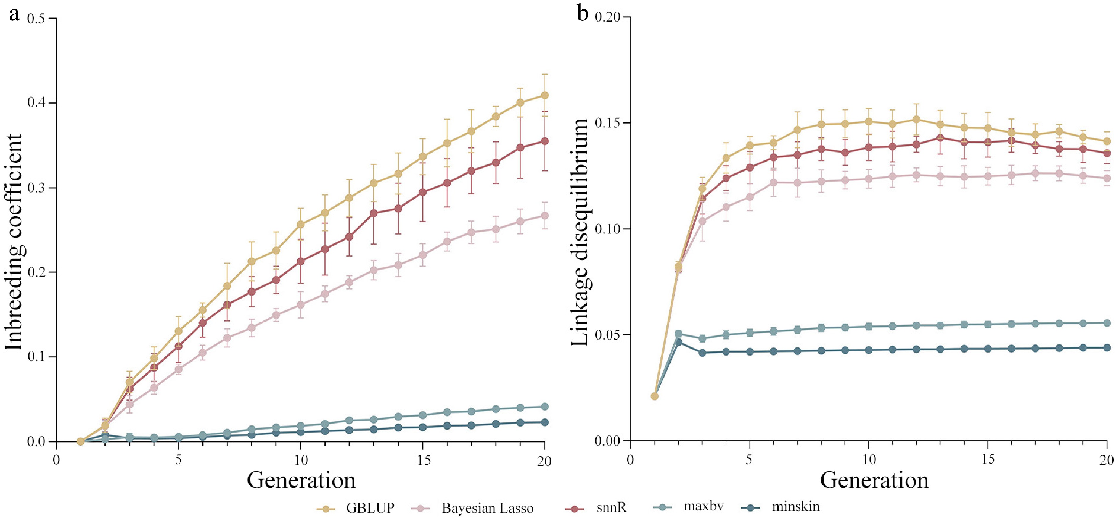
Figure 5. 

(a) Genomic inbreeding coefficient, and (b) linkage disequilibrium of genomic mating (GM) and genomic selection (GS) schemes in all generations.

The LD of the three GS schemes was considerably higher than that of the GM schemes, and the LD of all schemes was higher than that of the first-generation group (Fig. 5b). The LD of both 'maxbv' and 'minskin' showed an upward and then downward trend in the first 5 generations. By generation 20, LD of 'maxbv' decreased by 60.68%, 55.15%, and 59.05% compared to GBLUP, Bayesian Lasso, and snnR, respectively; LD of 'minskin' decreased by 68.98%, 64.62%, and 67.70% compared to GBLUP, Bayesian Lasso, and snnR, respectively. In the GS schemes, GBLUP had the highest LD while Bayesian Lasso showed the lowest. In GM schemes, LD of 'minskin' was 21.11% lower than that of 'maxbv'.

Among five breeding strategies, the 20^th-generation simulated population obtained under the 'maxbv', which aimed to maximise genetic gain while controlling the inbreeding coefficient, was selected for genetic structure analysis and comparison with the initial population. The results showed that the CV exhibited a continuous downward trend, and the individual components displayed no obvious stratification (Supplementary Fig. S4).

Computing efficiency

A comparison of the running efficiencies of all the schemes showed that the total running times across ten replicates of GBLUP, Bayesian Lasso, and snnR were 1,053.3, 1,193.5, and 1,095 min for 20 generations of simulation, respectively. The total running times across ten replicates of 'maxbv' and 'minskin' were 1,253.2 and 1,349.8 min for 20 generations of simulation, respectively, with the same CPU-based computational resources. Both GM schemes took more running time than GS schemes, with the most efficient being GBLUP and the least efficient being 'minskin'.

Population studies can help understand the domestication process of A. japonicus as well as the evolution of population structure and assist in breeding selection. In this study, the initial population was analyzed for genetic structure and parameters. Both PCA result and admixture result reflected that the initial population could be divided into Russian and Chinese populations based on genotypic data, which was consistent with the results of the manual sampling records. LD decay results indicated a high level of genetic diversity in the initial population. The maintenance of genetic variation is essential for the long-term survival of populations, and species with higher levels of variation are most likely to show high additive genetic variation in traits of interest^[38], which would greatly benefit the breeding of A. japonicus. Dominant effects have been demonstrated to have a certain impact on traits^[39]. The reliability of the model for estimating additive and dominant effect values was also demonstrated by the reliable simulated phenotypes obtained after incorporating dominant effect values in the model. Consequently, the initial population in this study had the breeding potential to meet the needs of multigenerational breeding.

Nevertheless, with prolonged artificial selection, genetic variability in breeding populations reduces with decreased genetic diversity^[40]. The core of GM is to achieve, as far as possible, the best possible trade-off between the conflicting goals of maximising genetic gain and maintaining genetic diversity.

GS strategies

GS results indicated that from the initial generation to the 20^th generation, all the schemes showed a trend of increasing followed by decreasing genetic gain. Among them, GS schemes showed a transient rise in genetic gain only in the very early generations, which is in line with current findings that, in the short term, inclusion of GS in breeding programs may accelerate genetic gains^[41]. On the other hand, the majority of the discussion on the long-term effects of GS is still at the stage of modeling studies. As GS ranked candidates on GEBVs and truncated the distribution to select those with the highest GEBVs, genetic gain increased, but so did inbreeding rates per generation. The reduction in genetic variance caused by a high inbreeding rate might result in detrimental long-term consequences, such as the fact that monogenic recessive alleles drift to high frequencies, causing disease^[42]. In general, as a truncation selection approach^[6], GS ignores the role of mating and complementation as evolutionary forces, which can lead to a reduction in genetic diversity and allelic purification after multiple generations of selection, and even inbreeding depression, limiting the long-term gain^[7].

Consequently, the progeny produced by the parents with the highest GEBV selected by the three GS schemes had increased inbreeding coefficients accompanied by a loss of additive genetic variance and reduced genetic diversity, thus preventing a substantial long-term genetic benefit^[43]. Under high-intensity truncation selection in GBLUP, the contribution of a few individuals with high GEBVs was disproportionately large, resulting in high inbreeding levels and low heterozygosity in progeny. The strong degree of LD and the homogeneous combination of alleles diminished the adaptive capacity and evolutionary potential of the population. Bayesian Lasso assumes that the trait-related marker effect variance can occur in the form of maximum and minimum values^[27], thus reducing allelic homogeneity in probability, resulting in a lower inbreeding coefficient and LD than GBLUP, and consequently, higher long-term genetic gain. Neural networks (NNs) are emerging as potentially powerful tools for genomic prediction of complex quantitative traits due to their ability to simultaneously account for non-linear relationships between molecular markers and QTLs^[44]. As a non-linear model with what is currently perceived as black-box behavior^[45], neural networks (NNs) cannot be used to derive interpretable conclusions about the influence of SNPs on phenotypes. The difficulty lies in discerning which features, and which combinations of features, the model has learned^[5]. The snnR model used in this study obtained moderate genetic gain and inbreeding coefficient among the GS schemes, which can be attributed to the fact that a sparsified neural network model is suitable for high-dimensional input variables and large sample sizes^[29], whereas the input genotype value data and sample sizes were low in this study, and the low complexity of the computation of the snnR limits it from capturing all the important genetic variants.

GM strategies

Inbreeding leads to an increased risk of losing favourable alleles and affects the potential for epistasis between dominant effects of heterozygous genes. Reductions in inbreeding can be achieved through simple management practices; however, these practices often come at the cost of reduced genetic progress. The importance of reducing inbreeding for long-term breeding has also been suggested by many investigators^[46]. These studies argued that GS may accelerate the decline in selection response unless new alleles are continually added; this emphasizes the importance of balancing short- and long-term gains by inbreeding in genetic selection. Achieving substantial long-term genetic gains requires a balance between selection and the maintenance of genetic diversity.

Different from GS, GM incorporates parameters such as kinship into breeding considerations, preserves the potential of each individual to contribute as a parent^[9], maintains sustainable genetic gain, and enables the selection of appropriate selection schemes according to different breeding objectives. In this study, we simulated 20 generations of simulated breeding with two breeding strategies, maximising breeding value and minimising kinship, using GM schemes based on the OCS algorithm. The results showed that although the two GM schemes differed slightly due to their respective optimization objectives, no significant differences were observed in either genetic gain or inbreeding coefficient, and both GM strategies outperformed the three GS schemes. The two GM strategies, although manifested in the form of maximising GEBV and minimising inbreeding coefficient, within the algorithms, each imposed restrictions on kinship and genetic contributions so as to achieve the core objective of GM^[31]. Therefore, the parameters employed in the GM models of this study fulfilled the core objective of GM, the balance between genetic gain and inbreeding. Genetic structure analysis of the population after 20 generations of GM breeding suggested that the 20^th-generation simulated population exhibited higher genetic diversity compared to the initial population. This result is consistent with the findings reported by Bérodier et al.^[47], which demonstrated that mating strategies incorporating genomic information can maximize genetic gain while maintaining substantial genetic diversity and minimizing inbreeding. When the breeding objective was to maximise the genetic gain for papilla number, it might lead to a positive gametic phase disequilibrium between QTL and polygenes^[48]. However, when the inbreeding coefficient was controlled simultaneously, selection would preserve the genetic diversity within the population and prevent any subpopulation from becoming dominant due to over-selection. Moreover, in simulated mating, free mating among individuals resulted in unimpeded gene flow, with each individual carrying multiple ancestral components^[49].

It has been reported that GOCS, restricting genomic relationships and weighted genomic selection, amplifying the effect of rare alleles, can enhance genetic gain but fail to prevent inbreeding and loss of rare variants. Maximising a weighted index balancing genetic gain with controlling expected heterozygosity or maintaining rare alleles resulted in superior long-term breeding simulations^[50]. Kang et al.^[34], on the other hand, proposed an open nucleus breeding system and a closed nucleus breeding system for simulating Pacific white shrimp, which increased genetic gain by introducing multiplier population individuals, but could not control the acceleration of inbreeding. The GM simulation breeding schemes proposed in this study achieve a trade-off, and it is believed that through data volume expansion, parameter optimization, and practical validation, GM will provide new insights into the molecular breeding of aquatic organisms.

Despite its potential benefits, GM still faces numerous challenges that need to be addressed. Ongoing research is essential to address the persistent challenges faced by GM and to enhance its applicability and impact. Research on GM in Holstein cows proposed that GM with non-additive genetic effects performed better than models with only additive effects. Mating programs with dominant and heterozygosity effects were better able to improve milk, fat, and protein yields^[39]. Tang et al.^[51] also demonstrated that genetic advantage from dominant effects can be used to maximise offspring performance in mate allocation. However, the dominant effect provided a slight contribution to phenotypic expression and, because of the low magnitude and amount of data available, the estimate of dominance variance was less accurate than that of additive variance^[39]. A significant portion of dominance variance might be confounded with environmental effects when dominant genetic effects were not considered^[52]. Dominance variance estimates might be inflated when models do not include genomic inbreeding, making an accurate estimate of marker effects critical for GM. Models for calculating dominant genetic variance that are closer to the true value in real breeding processes need to be improved. Assigning appropriate weights to markers to balance their genetic contributions, thereby improving the predictive performance of genomic selection, is an approach worth trying in GM as well.

In this study, the genetic architecture was simplified by assuming physically unlinked loci with purely additive effects. While this assumption facilitated the analysis of GM and GS strategies, it likely underestimates the genetic complexity of quantitative traits in reality. QTLs often exhibit LD and non-additive interactions, including epistasis, which can substantially influence trait expression and response to selection. By assuming unlinked loci, the model does not account for the Hill-Robertson effect, in which selection at one locus can interfere with linked loci, potentially accelerating the loss of favorable alleles.

Genotype by environment (G × E) interaction significantly impacted the prediction accuracy of GS models^[53]. Mas-Munoz et al.^[54] investigated the G × E interaction of sole reared in a recirculation aquaculture system and a semi-natural outdoor pond. The observation of heritable variation and low genetic correlation for sole growth across different environments indicates pronounced G × E interaction effects. The accuracy of selection and the predicted genetic gain might vary across different environments. Low genetic correlations implied that the optimal genotypes differed between environments. Therefore, differences among environments may have implications for breeding programs, and optimizing breeding programs in the presence of G × E interactions may maximize genetic gain across all environments^[55]. In this study, the calculation of environmental effects was simplified, which may not fully capture the complex G × E interactions and stochastic environmental noise inherent in real-world breeding systems. In practice, higher environmental variance could potentially reduce the accuracy of GEBVs, thereby impacting the optimization efficiency of GM. Thus, incorporating G × E interaction into GM models is highly anticipated. Introducing heterosis and breed-specific QTL effects in GM is also an interesting strategy^[56].

Furthermore, the simulation in this study did not explicitly incorporate overlapping generations, variation in reproductive success, or skewed sex ratios, which are intrinsic features of many aquaculture species like A. japonicus. In real breeding programs, these factors significantly increase the variance of long-term genetic contributions among individuals, often leading to a more rapid decline in effective population size than observed in discrete-generation models^[57]. For instance, skewed reproductive success can limit the pool of available high-ranking candidates, which may introduce additional constraints on mate allocation and potentially bias the expected genetic gain of GM schemes. While our study demonstrated the inherent advantages of GM in balancing gain and inbreeding, these findings still need to be further verified under more realistic conditions, such as by incorporating these complex biological variables into future stochastic simulation frameworks.

The 'maxbv' scheme, while maximizing immediate gain, may lead to the rapid fixation of alleles in specific family lines, potentially narrowing the genetic base for traits not included in the current selection index^[58]. On the other hand, the practical implementation of 'minskin' requires exhaustive pedigree or genomic kinship tracking of all candidates, which significantly increases genotyping costs. In aquaculture systems with high fecundity but high larval mortality, the actual number of contributing parents often deviates from the optimized mating design, a factor that could erode the theoretical advantages of GM observed in this study^[59].

With the explosive increase of genotype data and a large amount of phenotype data, running efficiency has become a concern for researchers. The results of this study showed that the running efficiencies of GM schemes were generally lower than the GS schemes, which may be due to the fact that the genetic contribution of parents and kinship were calculated in the GM^[32,33], thus increasing the amount of computation. It has been demonstrated that GPU-based computation could improve the runtime performance of the integration of multi-dimensional datasets by almost four orders of magnitude and was able to greatly accelerate the detection of genome-wide SNP-SNP interactions^[60]. Therefore, the use of a GPU for GM program through algorithm design and hardware optimisation may improve computational efficiency.

The genomic mating breeding approach provides a feasible method to balance genetic gain and genetic diversity, thereby achieving sustainable long-term genetic improvement. In this study, we conducted a 20-generation simulation study using genotype data of A. japonicus and simulated phenotype data for the number of papillae. We observed the performance of the papilla number under three GS and two GM strategies. The results demonstrated that the GM approach, while maximizing genetic gain, could control the level of inbreeding within certain limits, thus maintaining sustainable genetic improvement and achieving multi-objective targeted breeding. Compared to the GS strategy without controlling inbreeding, the GM strategies showed superiority in long-term breeding of A. japonicus. The study on genomic mating for the papilla number trait in A. japonicus reveals the broad prospects of genomic mating in aquaculture breeding applications. However, this study only focused on a single trait and used a specific heritability setting, so the findings may not directly apply to multi-trait breeding or traits with different heritabilities. Furthermore, this work was limited to computer simulations constrained by software settings and simplified assumptions, which cannot fully capture the complexities of practical breeding scenarios. Therefore, further experimental validation is needed in future studies.