Variations in proximate composition and energetic values among marine fish from South Pacific islands

Determining the proximate composition and energetic value of fish is important from two complementary perspectives: understanding fish bioenergetics and ecosystem functioning, and assessing their nutritional value for humans. From an ecological and physiological perspective, these measurements provide insight into how fish acquire, store, and allocate energy to key biological processes, including maintenance, locomotion, prey capture, growth, and reproduction. They can also inform estimates of energy transfer among trophic levels, thereby contributing to a better understanding of aquatic ecosystem dynamics and functioning^[1−3]. From a human nutrition perspective, the proximate composition and energetic value provide information on the nutritional quality of fish (proteins, lipids, etc.) and the amount of dietary energy they provide to humans. The latter perspective motivates the present study. Malnutrition (e.g., undernutrition, micronutrient deficiency, obesity) currently affects more than one-third of the human population. Although no region is unaffected, malnutrition is especially high in many tropical developing countries. Both a cause and a consequence of demographic pressure, social and economic inequalities, and the unsustainable exploitation of natural resources^[4], nutrition issues represent one of the greatest global health challenges of our century^[5]. Coastal communities, especially in developing countries, often rely on local artisanal fisheries and subsistence catches for a substantial share of their food supply and nutritional security. This is particularly true for people in Pacific Island countries and territories (hereafter, PICTs), which maintain strong environmental and cultural connections to marine resources^[6], and often have limited access to arable land and few opportunities to develop land-based agriculture or livestock production. Worldwide estimates indicate that fish contribute to ~15%–20% of total animal protein consumed globally^[7]. By contrast, in many PICTs, fish intake is two to four times the worldwide average^[8], contributing up to 90% of animal protein intake^[9]. Coastal reef fish represent approximately 70%–75% of the species consumed, with the remainder consisting primarily of tuna species^[10]. Annual fish consumption can reach 120–150 kg per capita in some Pacific Island communities^[11], while local fisheries may target several hundred species^[12].

Despite a growing number of studies focusing on the micronutrient composition of tropical coral reef fishes, including iron, zinc, vitamins, long-chain ω-3 and ω-6 polyunsaturated fatty acids, among other nutritional compounds^[13−16], comparatively little attention has been paid to quantifying and comparing their proximate compositions (i.e., proteins, lipids, and carbohydrates) and energetic values with those of terrestrial food sources. However, macronutrient composition, particularly proteins and lipids, directly determines the energetic value of fish. This is particularly relevant where diets rely heavily on starchy staples and/or ultra-processed imported food^[17]; fish is one of the few accessible and often cheap animal-source foods, thus detailed nutritional information of species could guide public policies on sustainable fisheries management and nutrition recommendations in different PICTs.

This study aimed to determine the proximate composition and energetic values of marine fishes from four South Pacific islands, focusing primarily on shallow coral reef species while also including a small number of pelagic and deep-water species. To our knowledge, comparable data on proximate composition and energetic values remain scarce in the South Pacific. We therefore compared our findings with those reported from other regions to assess potential biogeographical variation. We also tested whether proximate composition and energetic values differed among islands and trophic categories.

This study was conducted on 204 fish individuals, belonging to 46 species from 17 families. Fish individuals were collected by local fishermen in Fiji (October 2022, 60 fish from 19 species); Moorea (French Polynesia, November 2022, 65 fish from 17 species); New Caledonia (May–June 2023, 50 fish from 18 species); and Rapa Nui (i.e., Easter Island, November 2023, 29 fish from 13 species) (Table 1). For each site, the time interval between each sample collection ranged from 1 to 3 d, with four to five consecutive samples collected. Only New Caledonia showed slightly more variability in sampling, with seven samples collected over a period of about 20 d. All fish are from coral reefs, except in Rapa Nui, where some individuals were caught from deep and pelagic ecosystems. Sampling was conducted to obtain a wide range of fish species with contrasting feeding strategies. However, fishermen were unable to guarantee homogeneous catches, thus resulting in unbalanced sampling, with some species being represented by only one individual whereas some others were represented by up to eight individuals, although having a homogeneous size range within each species (Table 1). These species, even the smallest ones (such as Holocentridae at Rapa Nui, for instance; see Results section), are frequently caught by fishermen, thus reflecting their consumption by local human communities. Fish species were categorised into three broad trophic groups: herbivores (mainly consuming macrophytes), omnivores (consuming both animal and plant material), and carnivores (consuming animal prey). In all cases, fish were kept in coolers, and each individual was identified and measured (total length, in cm). For each fish, samples of white dorsal muscle were taken (~15–20 g fresh wet weight) and immediately frozen at −20 °C.

Analysis of proximate composition

The first step was to measure the wet weight (ww) of the samples and then to freeze-dry them for 48 h. The dry weight (dw) of the freeze-dried samples was measured, which allowed us to calculate the % moisture. In a second step, dry samples were ground into a fine powder, and subsamples of this powder were used to quantify the protein, carbohydrate, and ash contents. The lipid content was then calculated as the difference between the total dry mass and the sum of protein, carbohydrate, and ash contents.

Determination of protein % was performed using the colorimetric method developed by Lowry et al.^[18] which has the advantages of being relatively sensitive and not requiring prior digestion of the proteins, which facilitates the process. This method is based on two reactions that lead to the formation of a blue-coloured complex. The first reaction involves reacting the proteins with an alkaline copper reagent, thereby forming a protein-copper complex. The second reaction involves Folin–Ciocalteu's reagent. This reagent, when mixed with the protein-copper complex, reduces the aromatic amino acids, generating a dark-blue complex. The intensity of the colour is proportional to the amount of protein and is measured by a spectrophotometer (Perkin-Elmer®, Lambda XLS) at 700 nm and compared to a control. In the first reaction, 10 mg (dw) of fish powder was diluted in 10 mL of water and homogenised. A volume of 0.3 mL of this solution was put into a centrifuge tube, and a volume of 5 mL of cupric reagent was then added. This cupric reagent is made up of 100 mL of 2 g of sodium carbonate (Na₂CO₃) dissolved in 100 mL of 0.1 M NaOH, plus 1 mL of 0.5% CuSO₄ copper sulphate solution, plus a 1% sodium tartrate solution. After homogenisation and a pause of 20 min, the second reaction is run by adding 0.5 mL of Folin–Ciocalteu reagent. The solution is then left standing for 30 min in the dark to allow the colour to develop. This solution was then centrifuged for 20 min at 1,500 rpm to clarify the supernatant for colorimetric measurements. A 300 μL volume of supernatant was recovered and placed in a microplate to measure absorbance using a microplate reader (BioTek®, Epoch 2) at 700 nm. Each sample was analysed in three replicates to ensure the reliability of the measurements. The same protocol is applied to solutions of bovine serum albumin at different known concentrations to establish a calibration line. The absorbance values are then plotted against the calibration line. The protein concentration is determined by the following formula: (P) = (Abs−b)/a, where (P) represents the protein concentration in mg/mL, Abs is the absorbance at 700 nm, a is the slope of the calibration line, and b is the intercept of the calibration line. The protein concentrations are then converted into percentages per 100 g of fish, i.e., %ww.

Carbohydrate contents were often neglected in the determination of proximate composition in fish because the carbohydrate % is usually < 1% in wet weight^[19,20], although a value around 3% was reported for Clupea fimbriata in Malaysia^[21]. However, to our knowledge, such data do not exist for tropical coral reef fish, and we then conducted such carbohydrate analyses on our samples. We used an adaptation of the colorimetric method of Dubois et al.^[22] which is based on the reaction between carbohydrates, concentrated sulphuric acid, and phenol. A 10 mg (dw) mass of powder from each sample was taken and diluted in 5 mL of distilled water. A volume of 0.5 mL of this solution was then taken, to which 0.5 mL of distilled water was added to ensure proper dilution, and 0.5 mL of 5% phenol was added, followed by the addition of 2.5 mL of 98% concentrated sulphuric acid, and the tubes were then placed in an ice bath. Sulphuric acid dehydrated the carbohydrates in the sample, which then reacted with the phenolic compounds to form a yellow-coloured complex. This colouration is proportional to the quantity of carbohydrates present in the sample, making it possible to estimate their concentration. The tube containing the reaction mixture is then placed in an oven for 30 min at 45 °C, ensuring a complete reaction between the components and the formation of a stable-coloured complex. After incubation, the absorbance of the solution is measured at 490 nm using a spectrophotometer (Perkin-Elmer®, Lambda XLS). The values obtained are then compared with a calibration curve based on standard glucose solutions of known concentrations. Thus, the carbohydrate concentrations can be estimated using the calibration line formula, as follows: (C) = (Abs−b)/a, where (C) is the carbohydrate concentration in mg/mL, Abs is the absorbance at 490 nm, a is the slope of the calibration line, and b is the y-intercept of the line. The percentage of carbohydrates in wet weight is then calculated by relating this concentration to 100 g of fish.

Determination of ash content resulted from calcinating freeze-dried powder. Approximately 0.2 g of powder from each sample was placed in previously tared porcelain crucibles and then placed in a muffle furnace at 500 °C for 4 h. Calcination eliminates the organic fraction of the sample, leaving only the mineral part, i.e., the ash. The crucibles were then cooled in a desiccator to prevent them from regaining moisture and weighed to determine ash mass.

Finally, the % of lipids content (ww) was simply determined by subtracting the % of moisture, proteins, carbohydrates, and ash from 100.

Data analyses

Energetic values were calculated from the measured proportions of protein, lipids, and carbohydrates using conversion factors of 23.6 kJ·g⁻¹ for protein, 39.56 kJ·g⁻¹ for lipids, and 17.2 kJ·g⁻¹ for carbohydrates^[23,24].

Principal component analysis (PCA) was performed on proximate parameters (moisture, proteins, lipids, carbohydrates, and ash) as a function of trophic categories and study sites. Differences in composition between islands or diets were analysed using analysis of variance (ANOVA). For each case, the model calculated the coefficient of determination (R²), which indicated the percentage of variation in the parameter to be modelled (energetic values, moisture, proteins, etc.) that is explained by the explanatory variables (site or diet). The closer this coefficient is to 1, the better the model, whereas the closer it is to zero, the poorer the model. For the few species sampled in at least two sites (with n ≥ 3 in both sites), Mann–Whitney tests were run to determine the statistical differences between islands for proximate parameters and energetic values. All these analyses were carried out using XLSTAT (free version).

The first two axes of the PCA explained ~75% of the global variation (Fig. 1). Although a wide overlap was evident between trophic categories, fish from various trophic groups (i.e., carnivores, herbivores, and omnivores) showed some differences (Fig. 1a). For instance, carnivores displayed a wide dispersion along axis 1, mostly driven by moisture and proteins, whereas herbivores showed a moderate dispersion, mostly along axis 2, driven by lipids and ash. Similarly, fish from the sampled sites (i.e., the four investigated islands) also displayed some differences, although only fish from Rapa Nui appeared more distinct from each other than those from the other islands (Fig. 1b).

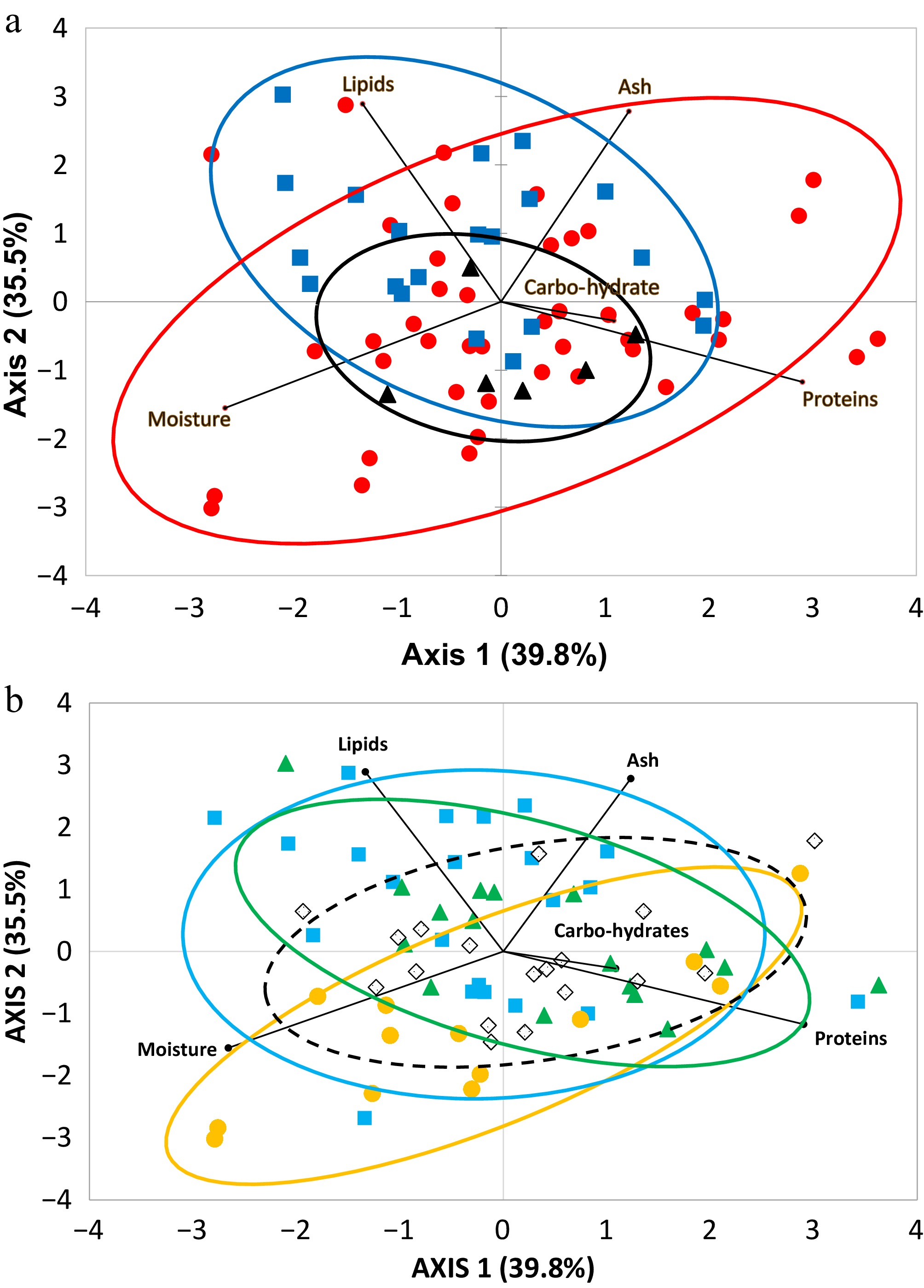
Figure 1. 

Biplot of the principal component analysis (PCA) run on proximate composition parameters of (a) carnivores (red circles), herbivores (blue squares), and omnivores (black triangles) fish, all sites pooled, and (b) on fish from Fiji (pale blue squares), Moorea (green triangles), New Caledonia (white diamonds), and Rapa Nui (orange circles), all diets pooled.

Moisture % was by far the most important component of fish flesh (78.1% ± 1.7% ww on average) and ranged from 73.5% (Atule mate from New Caledonia) to 83.3% (Sargocentron wilhelmi from Rapa Nui) (Table 2). Proteins constituted the second most important component (16.1% ± 2.3% on average) and ranged from 11.3% (Acanthurus triostegus from Moorea) to 22.0% (Rastrelliger kanagurta from Fiji); followed by lipids (4.4% ± 1.7% on average) that varied from 1.9% (Carangoides equula from Rapa Nui) to 8.5% (Lutjanus bohar from Fiji) (Table 2). Ash constituted a low fraction of fish flesh (1.2% ± 0.2% on average) and fluctuated from 0.7% (Acanthistius fuscus from Rapa Nui) to 1.5% (Parupeneus barberinus from Fiji). Finally, carbohydrates represented a very low percentage of fish ww (0.15% ± 0.07% on average) and ranged from 0.03% (Ctenochaetus striatus from Fiji) to 0.49% (Acanthurus dussumieri from New Caledonia) (Table 2). The energetic values ranged from 3.99 kJ·g⁻¹ ww for S. wilhelmi at Rapa Nui to 6.81 kJ·g⁻¹ ww for A. mate in New Caledonia (Table 2).

Fluctuations in proximate composition (moisture, lipids, etc.) and energetic values remained generally small from one island to another (Table 3). Although spatial fluctuations were statistically significant, the R² values were low in all cases, reaching a maximum of only ~30% for carbohydrates, the least abundant compound, and were ~7%–17% for key compounds (moisture, proteins, and lipids) (Table 3). Overall, fish from Rapa Nui differed most markedly from those sampled at the other islands, except in their protein and carbohydrate contents. Proximate composition and energetic values among trophic categories were also close to each other, and the R² values indicated either significant but weak variations in some cases (proteins, lipids, ash, energetic values) or non-significant variations for two other cases (moisture, carbohydrates) (Table 3). Overall, herbivores contained significantly less protein than omnivores and carnivores (~15% vs 17%, respectively), and the opposite was observed for lipids (~5.3% vs 3.7%) (Table 3).

For the seven species analysed in at least two sites, most spatial differences in proximate parameters and energetic values were statistically non-significant, despite few exceptions such as for Naso unicornis, Scarus rivulatus, and R. kanagurta for proteins and lipids (Table 4).

In tropical coral reefs, many fish species showed energetic values within the approximate range of 3.4 to 6.8 kJ·g⁻¹ for raw edible tissue (i.e., white muscle)^[14]. Overall, despite some variation in certain compounds (proteins or lipids, for example), the proximate composition and energetic values of the different species examined here were broadly consistent with values reported from the Red Sea^[25], the Gulf of Oman^[26], Malaysia^[21], and Sri Lanka^[27]. Similar results were also found in temperate ecosystems, such as in Turkey^[28], the Azores archipelago^[29], and even in cold waters such as the Patagonian^[20] or Arctic regions^[1,30]. However, fish from upwelling or other high-productivity temperate or cold-water zones usually reach higher lipid levels than conspecifics or species having a similar diet in tropical reefs^[31,32], which often implies a higher mean energetic value because the conversion ratio into energetic value is higher for lipids than for proteins.

Thus, and despite differences between species and/or between sites, etc., there is no doubt that in all cases and, unsurprisingly, fully in line with a recent review^[33], moisture is by far the major component of fish flesh, followed by proteins and lipids. Ash always accounts for a minimal proportion, while carbohydrates are marginal at best. Our results clearly pointed in this direction and confirmed the very low percentage of carbohydrates, which was to be expected, including for coral reef fish.

Although this general trend is well established, several types of fluctuations in proximate composition parameters and energetic values were reported by several studies, depending, for instance, on seasonal variations in fish physiology, changes in local environmental characteristics, and the sex and/or age of individuals. Our sampling design did not allow us to assess seasonal physiological variations, as samples were collected in austral winter in New Caledonia and in early spring at the other sites. However, because these consecutive seasons are only weakly contrasted in tropical South Pacific waters, the sampling season was unlikely to be a major source of variation in our dataset. However, seasonal variations in sexual maturation and breeding periods can have very significant effects on proximate composition parameters, through the mobilisation of muscle lipids and proteins as a source of energy for gonadal maturation and spawning^[34,35], and sometimes for long-distance migrations in migratory species such as salmon, for instance^[36].

Sex and age were also not studied in this work, although several studies have highlighted the importance of these two biological parameters on proximate composition^[1,3,27]. For instance, Ball et al.^[1] argued for an increase in energetic value with individual fish length due to an associated increase in body size, a reduction in body water stores (i.e., % of moisture) with growth, and a shift in the allocation of resources from growth (i.e., mostly proteins) to storage (i.e., lipids). Fish length can serve as a proxy for age, although this relationship becomes less reliable in older individuals because somatic growth slows as fish approach their species-specific asymptotic size. In our study, individuals of each species collected at a given site generally fell within a narrow size range (Table 1), suggesting limited variation in body size and, most likely, life stage within species. Consequently, ontogenetic variation in diet and in the assimilation of dietary proteins and lipids was unlikely to be a major source of variation in our results. Nevertheless, because fish were not directly aged, a residual effect of age cannot be excluded. To our knowledge, the role of sex in proximate composition has often been overlooked. In a study of three coral reef mesopredator species in Sri Lanka (one grouper, one snapper, and one emperor), Edirisinghe et al.^[27] showed significant differences in energetic values, protein, and lipid contents between males and females. However, there is no unequivocal link between these results and a sampling period that would correspond to gonadal maturation and/or spawning in this region, except for the grouper (Epinephelus merra). It therefore remains difficult to draw clear conclusions about male vs female differences and reproductive status, and further research is needed to investigate this important aspect of fish biology.

Local environmental characteristics depend on multiple parameters (pelagic productivity, algal and living coral cover, three-dimensional structure of the benthic substrate, natural and anthropogenic pressures, etc.), which themselves govern the diversity, abundance, distribution, and then availability of food resources for fish. Although these aspects were not investigated in this study, it is interesting to note a certain similarity in the proximate composition parameters and energetic values, even though the coastal environments differ from one site to another. The most notable case is that of Rapa Nui, which has a coastal environment that is depauperate in marine fauna compared to the other Pacific sites studied^[37−39], lower mean SST^[40], hyper-oligotrophic waters^[41], and a context of pronounced oceanic isolation^[42]. This situation might in part explain some of the results found at that site. For instance, the lower mean energetic values in Rapa Nui compared to the three other islands resulted from differences in biochemical composition (more moisture, less lipids), possibly because some species from that island were not all related to coastal reefs, but rather to deeper (e.g., A. fuscus) and pelagic ecosystems (e.g., Xiphias gladius) (Table 2). In fact, low lipid content in highly migratory species such as swordfish X. gladius could be attributed to starvation periods linked with its reproductive cycle^[43]. However, except for Rapa Nui, it remains difficult to draw general conclusions regarding energetic values, as the maximum and minimum values show no particular pattern, either spatially or in terms of taxa (family or species level). For example, within the Carangidae family, we found one of the species with the highest energetic values (A. mate) and one of the lowest (C. equula). In all cases, the differences between the minimum and maximum values are close to 2 kJ·g⁻¹ at best (something found in certain low-caloric vegetables), corresponding to a modest difference in energetic intake. It is therefore reasonable to suggest that the differences we observe between minimum and maximum energetic values are likely to have little nutritional impact.

All species examined in this study are caught at the four study sites by local small-scale fisheries, both for sale and for subsistence consumption^[12], highlighting their economic and nutritional importance to coastal communities^[8]. The lower energetic value of tropical reef fish (due to their lower % of lipids) compared to oily temperate fish makes them potentially less valuable in diets where caloric intake is limited, but had the advantage of supplying abundant protein without high fat intake^[13]. In PICTs, reliance on coastal reef fishes for protein is extremely high^[6,8,11]. Consequently, declines in fish stocks, whether driven by natural or anthropogenic factors, could reduce dietary energy adequacy in these communities, particularly in PICTs where alternative energy-dense foods may not be readily available. But there are exceptions for certain food products that are relatively easy to obtain locally (i.e., non-imported) and most commonly used in PICTs, such as tubers (taro, yam, manioc), eggs or chicken, and sometimes, in more restricted places, pork or beef.

Tropical coastal reef fishes represent nutritionally valuable protein sources that are broadly comparable to egg, chicken, and pork (in the latter case, depending of its lipid content) in macronutrient composition. They typically contain ~15–20 g protein and ~2–6 g lipids per 100 g edible portion, yielding 3.4 to 6.8 kJ·g⁻¹ (fresh flesh). Compared to temperate oily fishes (e.g., herring, sardine, anchovy, salmon), tropical reef fishes usually display lower energetic values but still provide high-quality protein and important micronutrients^[13−16]. For PICTs' human coastal communities, reef fishes are absolutely indispensable as sources of protein, not only through their lower energy contribution, implying that complementary calorie-rich staples and other food sources are key, but also through their ease of capture (proximity to coral reefs; methods used are often cheap and rudimentary, etc.).

The differences in proximate composition and energetic values identified in this study remain globally modest at the spatial scale studied. This could allow for a cautious extrapolation of our results to most fish species at the scale of the South Pacific Ocean basin. These findings are of interest in terms of human nutrition and the management of small-scale fisheries. From a nutritional perspective, our results suggest that there is no strong argument for favouring one category of species over another solely on the basis of energetic values. As local coastal fisheries most often target hundreds of species^[12] and often in an opportunistic manner, our results support this type of fishing strategy. This hypothesis needs to be tested in future research, which should also address the role of species-specific variability in proximate compounds according to age, sex, sexual maturity, and nutritional composition of diets, across multiple seasonal and environmental settings, as well as on broader proteins (i.e., amino acids) and lipids (notably ω-3 and ω-6 polyunsaturated fatty acids) profiles of tropical coastal reef fishes. Given the ongoing pressures of overfishing, degradation of coastal habitats, and climate change, a better understanding of their nutritional role is crucial not only for food security but also for fisheries management and dietary planning in PICTs.