Research on site selection and collaborative dispatch for unmanned aerial vehicle logistics distribution centers

The sustained rapid development of the low-altitude economy and the urgent, high-demand requirements for last-mile logistics have created a practical need for unmanned aerial vehicles (UAVs) to deliver high-efficiency, point-to-point transport in complex terrain environments such as mountainous regions and urban-rural fringe areas^[1,2]. The escalating logistics demands in mountainous regions has exposed the inefficiencies and high costs inherent in traditional ground transport, constrained by topography and infrastructure limitations. Conventional ground transport systems significantly extend routes, time, and costs when navigating complex terrain such as mountain ranges and river valleys. Furthermore, they may be restricted by road conditions and extreme weather, preventing the delivery of goods to remote villages and towns. Against this backdrop, both academia and industry have conducted in-depth research addressing issues such as how to deploy logistics distribution networks, how to operate drones, and how to control total costs.

Recent years have seen substantial progress in research on applying drones to logistics systems, with increasing focus on key technologies like hub siting and collaborative delivery. O'Kelly et al. conducted a meta-review on hub-and-spoke planning (HLP)^[3], highlighting challenges and opportunities for air/multimodal transport and sustainability in emerging scenarios. Meng et al.^[4] developed a location-route optimization model using blood delivery as a case study, jointly solving site location and UAV routing to validate drone value in time-critical medical logistics. Cavagnini et al.^[5] modelled location-route problem coverage. Regarding algorithmic approaches for problem-solving, a diverse array of optimization algorithms currently exist for site selection and route planning models, broadly categorized into four types: traditional algorithms, intelligent optimization algorithms, quantum algorithms, and machine learning algorithms^[6]. Traditional algorithms, grounded in deterministic logic, prioritize optimal path discovery within known topological structures. Representative methods include Dijkstra's algorithm^[7], RRT*^[8], and the A* algorithm. These approaches offer theoretical rigor, path stability, and computational precision, yielding globally optimal solutions for small-scale problems. However, they often incur high computational time costs when applied to high-dimensional, non-linear models with complex constraints. Collective intelligence optimization algorithms provide efficient tools for tackling such complex optimization problems. Jiang & Xu^[9] proposed the Particle Swarm Optimization-based Uniform Probability Rapidly Expanding Random Tree (PSO-PH-RRT*) algorithm, achieving significant improvements in path generation efficiency within three-dimensional dynamic environments. Meng et al.^[10]employed segmented chaotic mappings, adaptive t-distribution mutation, and dynamic weight adjustment strategies to construct the MSDBO algorithm, achieving an adaptive equilibrium between global exploration and local refinement. Chakraborty et al. conducted extensive research addressing issues in WOA, such as premature convergence, insufficient population diversity in later stages, and an imbalance between global and local searches. They systematically proposed multiple improvement methods, enhancing global exploration capabilities and accelerating convergence through mechanisms including chaotic mapping, non-linear adaptive weights, and increased perturbations. Multiple synergistic operators and local search operators were constructed to form a multi-strategy WOA, improving solution accuracy and stability. Furthermore, WOA was hybridized with other swarm intelligence algorithms such as GWO and SCA to develop hybrid WOA variants suitable for large-scale optimization, path planning, and engineering structural design scenarios^[11].

However, the research predominantly focuses on urban or flat terrain, approximating distance costs for distribution center siting using Euclidean distance, or road mileage on a two-dimensional plane. Consequently, evaluation outcomes deviate significantly from actual expenses. Compared to road networks, low-altitude airspace in mountainous terrain is influenced by multiple factors, including topographical undulations, no-fly zones, and altitude restrictions^[12,13]. Traditional models combining planar Euclidean distance with single-vehicle path planning struggle to accurately assess actual costs and frequently yield infeasible solutions under time window and capacity constraints^[14]. This paper addresses the location and collaborative scheduling problem for UAV logistics distribution centers within mountainous transportation systems. A two-layer Location Routing and Scheduling Problem (LRSP) model is constructed, encompassing intelligent site selection and flight path planning alongside task allocation and collaborative scheduling. The key sets, decision variables, and parameters used throughout the two-layer model are summarized in Table 1.

As shown in Table 1, the current dual-layer structure in vehicle research typically operates at the road and lane levels for trajectory control and risk management, without addressing the coupling of hub selection, time-window services, and three-dimensional airspace constraints in drone logistics. Meanwhile, the two-layer structure for drones is predominantly applied in urban scenarios, focusing on low-risk urban airspace and conflict avoidance. However, it often excludes safety altitude constraints imposed by mountainous terrain undulations, 3D trajectory costs, and the logistics LRSP closed loop at the dispatch layer.

Within the research framework of this paper, the base model employs IWOA to achieve solution optimization. It first solves for candidate hub locations by integrating factors such as spatial distance from task points to hubs, elevation-based operational costs, and transport costs weighted by task volume. During the site selection process, each potential hub location is scored to construct the comprehensive evaluation function of the location model. Using the selected distribution centers and known task point coordinates, IWOA generates feasible three-dimensional flight paths for any pair of nodes that satisfy terrain elevation and safety altitude constraints. The aggregated flight distances or energy consumption form the underlying trajectory cost matrix. The top-level model then employs an IALNS on the trajectory cost matrix provided by the base model to coordinate the scheduling of multiple UAVs' tasks, time windows, and payload constraints. This achieves unified optimization for multi-UAV task allocation in the three-dimensional flight path planning for distribution center siting. A schematic of the research model is illustrated in Fig. 1 below.

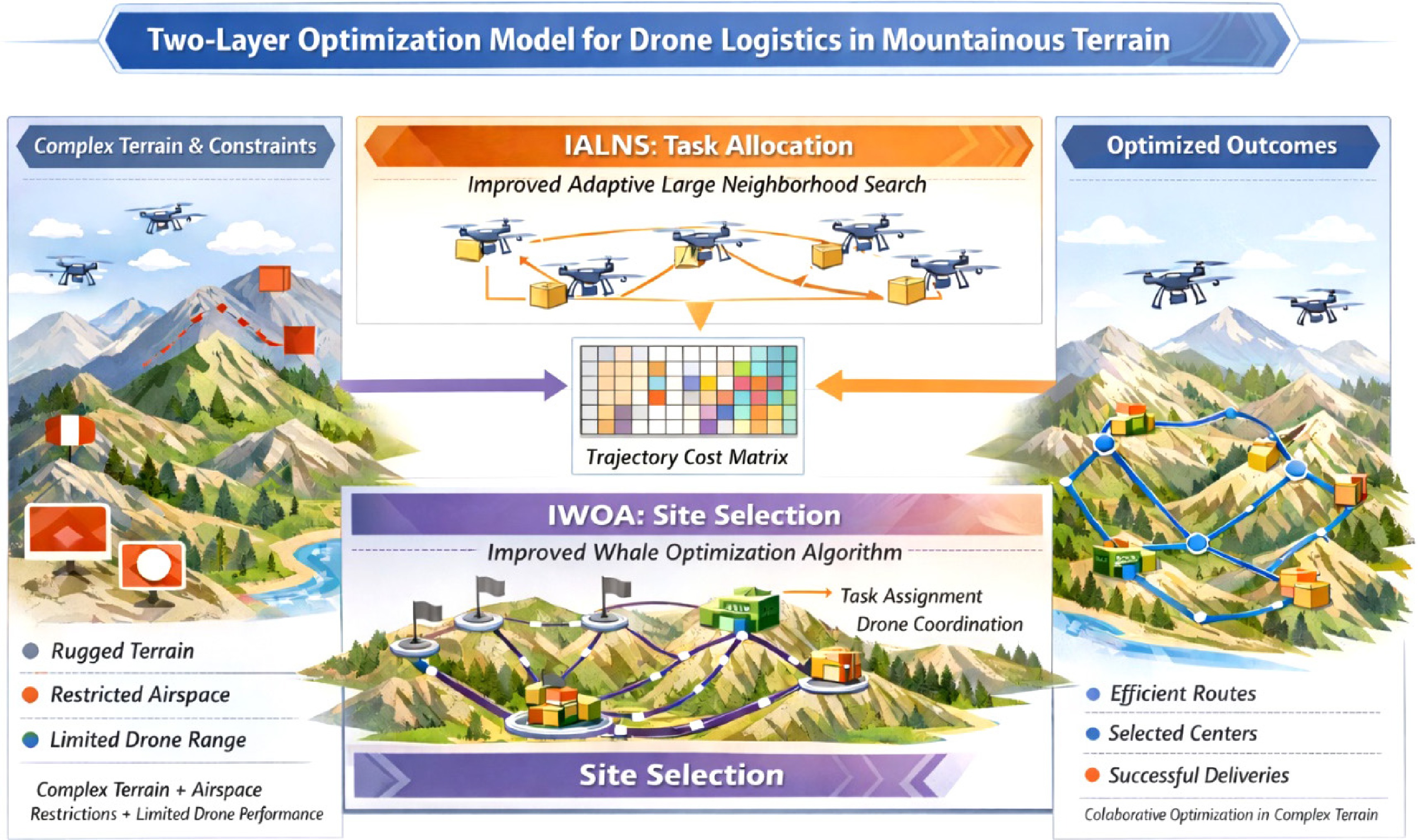
Figure 1. 

Research model diagram.

To characterize the collaborative optimization relationship between hub location selection, three-dimensional flight paths, and task allocation within mountainous drone logistics systems, this paper constructs a two-layer model for the Location–Routing and Scheduling Problem (LRSP). The model makes the following assumptions:

(1) A single-hub distribution model is adopted, where candidate hub locations may be situated at any point on a continuous terrain plane, provided they avoid no-fly zones and obstacles.

(2) The coordinates, delivery task volume, and time windows for each task point are known, and remain constant throughout the planning period.

(3) Each task point must be served by exactly one drone on a single occasion; each drone departs from the hub, executes its assigned task sequence, and must ultimately return to the hub.

(4) The upper and lower bounds of distribution center construction costs are known, as are the dispatch costs per drone.

(5) All drones are identical in type, possessing the same payload capacity, endurance, safety distance, pitch angle, and other parameters.

(6) An adequate number of drones are available; the optimal number required is determined by back-calculating from mission demands.

(7) Weather factors such as wind speed, thunderstorms, or smog are not considered.

Symbol legend

The variables and their meanings in this chapter are shown in Table 2.

Model construction

The rational siting of distribution centers helps to shorten service distances, enhance delivery efficiency, and reduce system operating costs. First, outer rectangles are constructed around all task points based on their planar coordinates. Subsequently, the entire area is expanded by 5% to obtain the candidate distribution center zone with an extended safety margin. Several initial distribution center locations $ \left({x}_{G},{y}_{G}\right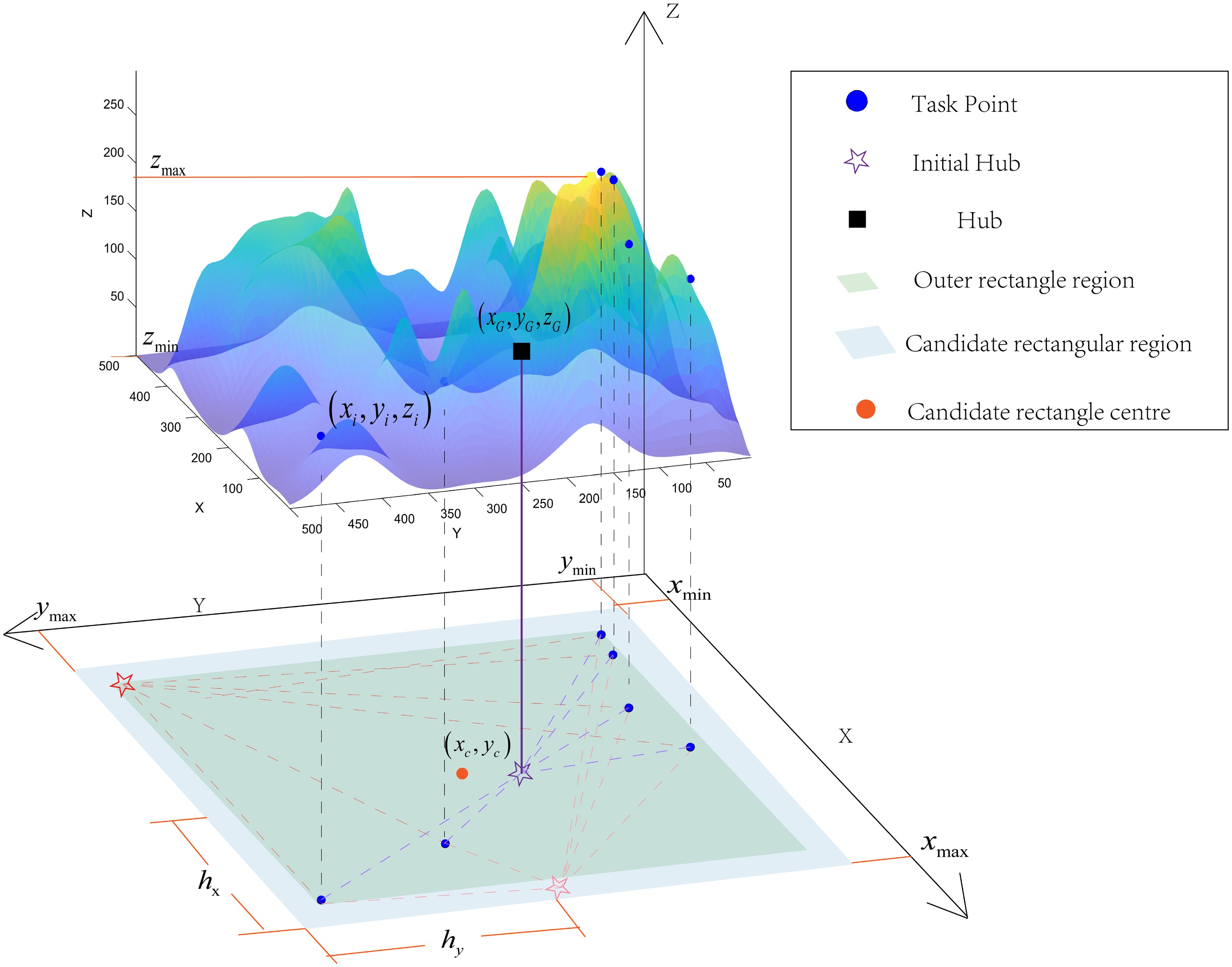) $ are then generated within this candidate zone. Employing a multi-start local search, through terrain interpolation, the operational maintenance costs for Site $ {z}_{G} $ are assessed to solve the site selection model. The evaluation criteria comprise the service distance from the distribution center to each task point, the elevation-related operational maintenance costs at the distribution center location, construction costs, and transportation costs based on task volume and service distance. Subject to site selection area and terrain constraints, the optimal solution with the lowest comprehensive cost is retained as the location for the UAV logistics distribution center. The distribution center selection model is illustrated in Fig. 2.

Figure 2. 

Hub selection schematic.

The mathematical model for site selection is shown in Eq. (1):

Where, $ H $ denotes the objective function for site selection, $ {H}_{Length} $ represents distance costs, $ {H}_{Elev} $ denotes operational and maintenance costs for the distribution center, $ {H}_{Build} $ denotes construction costs for the distribution center, and $ {H}_{Trans} $ denotes transportation costs, as shown in Eqs (2) to (5):

Eq. (2) represents the service coverage level of a distribution center relative to task points in spatial location selection. It averages the planar service distances from the distribution center to each task point to derive distance costs. A lower value indicates the distribution center is closer to the overall center of gravity of the task area, resulting in a shorter average service distance. Eq. (3) quantifies the impact of the distribution center's elevation on operational maintenance costs. In mountainous terrain, higher elevation typically entails greater long-term expenditures on equipment maintenance, site upkeep, and transport logistics. Therefore, the equation normalizes the distribution center's elevation within the minimum and maximum ranges of candidate areas, constructing a monotonically increasing operational maintenance cost function. This ensures that the distribution center's elevation is optimally positioned between these bounds. Equipment maintenance, site upkeep, and transport support incurs greater long-term expenditures. Therefore, the distribution center's elevation is normalized between the minimum and maximum heights within candidate areas, constructing a monotonically increasing operational maintenance cost function. This ensures higher elevations correspond to higher operational costs, thereby avoiding unnecessary high-altitude risks during distribution center selection. Eq. (4) represents the infrastructure investment required for establishing distribution centers at different locations. When a distribution center is situated near the geometric center of the task area, construction and material organization are relatively convenient, approaching the minimum cost; conversely, costs approach the maximum. Eq. (5) represents the operational expenses required for a drone to complete deliveries to all task points from a given distribution center location. Transport costs are jointly correlated with demand distribution and spatial distance distribution; they do not solely favor areas dense with task points, but also low in task volume. Therefore, operational expenses are calculated as the sum of the product of each task point's task volume and its service distance to the distribution center, serving as one of the core indicators for evaluating the economic viability of site selection schemes^[20]. Where $ {h}_{\mathrm{x}} $ and $ {h}_{y} $ denote the half-width and half-length of the rectangular boundary, respectively, representing the maximum distance attainable from the center of the region along the $ x $-axis or $ y $-axis towards the boundary of the rectangle. The offset $ \rho $ is defined as shown in Eqs (6) to (8).

Upon selecting the distribution center, the system performs trajectory planning and task allocation. The overall objective function is defined as shown in Eqs (9) to (11), with constraints as specified in Eqs (12) to (16):

Where, $ {F}_{Length} $ denotes flight distance cost, $ {F}_{Space} $ denotes spatial coordination constraint cost, $ {F}_{height} $ denotes flight altitude cost, $ {F}_{Threat} $ denotes threat zone cost encompassing sensitive areas, restricted airspace, and other high-risk zones; $ {F}_{Pitch} $ denotes pitch angle cost, $ {F}_{\text{timewin}} $ represents time constraint cost, and $ {F}_{load} $ denotes contract constraint cost. Eq. (12) ensures each mission point has exactly one service path while preserving traffic conservation; Eq. (13) guarantees each UAV takes off from the distribution center; and Eq. (14) ensures each UAV must return to the distribution center.

The results of the underlying three-dimensional flight planning is injected into the upper-level task allocation and scheduling model to form the final trajectory cost matrix. Therefore, the final trajectory cost $ S $ is as shown in Eq. (15):

Where, $ H $ and $ J $are defined by Eqs (1) and (9) respectively.

This paper employs a two-layer framework: the base layer centers on IWOA, independently optimizing three-dimensional flight paths between any two points—the center and individual task points—while integrating constraints such as terrain interpolation, safety altitude, no-fly zones, and smoothness. For each segment, it generates a flyable curve along with its arc length, subsequently aggregating these results. The upper layer integrates these outputs through an optimization process. Utilizing an IALNS, it rapidly screens high-quality feasible solutions within the large solution space, subject to constraints including capacity, time windows, mission uniqueness, and traffic balance. Throughout this workflow, data transmission proceeds from bottom to top, with clearly defined interfaces.

Improved Whale Optimization Algorithm, IWOA

To overcome the shortcomings of the traditional WOA when addressing high-dimensional complex problems, such as the imbalance between exploration and exploitation and the tendency towards local optima, this paper proposes an IWOA^[21,22]. The proposed IWOA algorithm introduces three enhancement modules. First, it employs adversarial population initialisation to enhance the diversity of initial solutions; second, a non-linear convergence factor facilitates a smoother transition between exploration and exploitation; and finally, an elite refinement mechanism based on genetic algorithms mitigates search stagnation, and improves local search precision. Its flowchart is illustrated in Fig. 3.

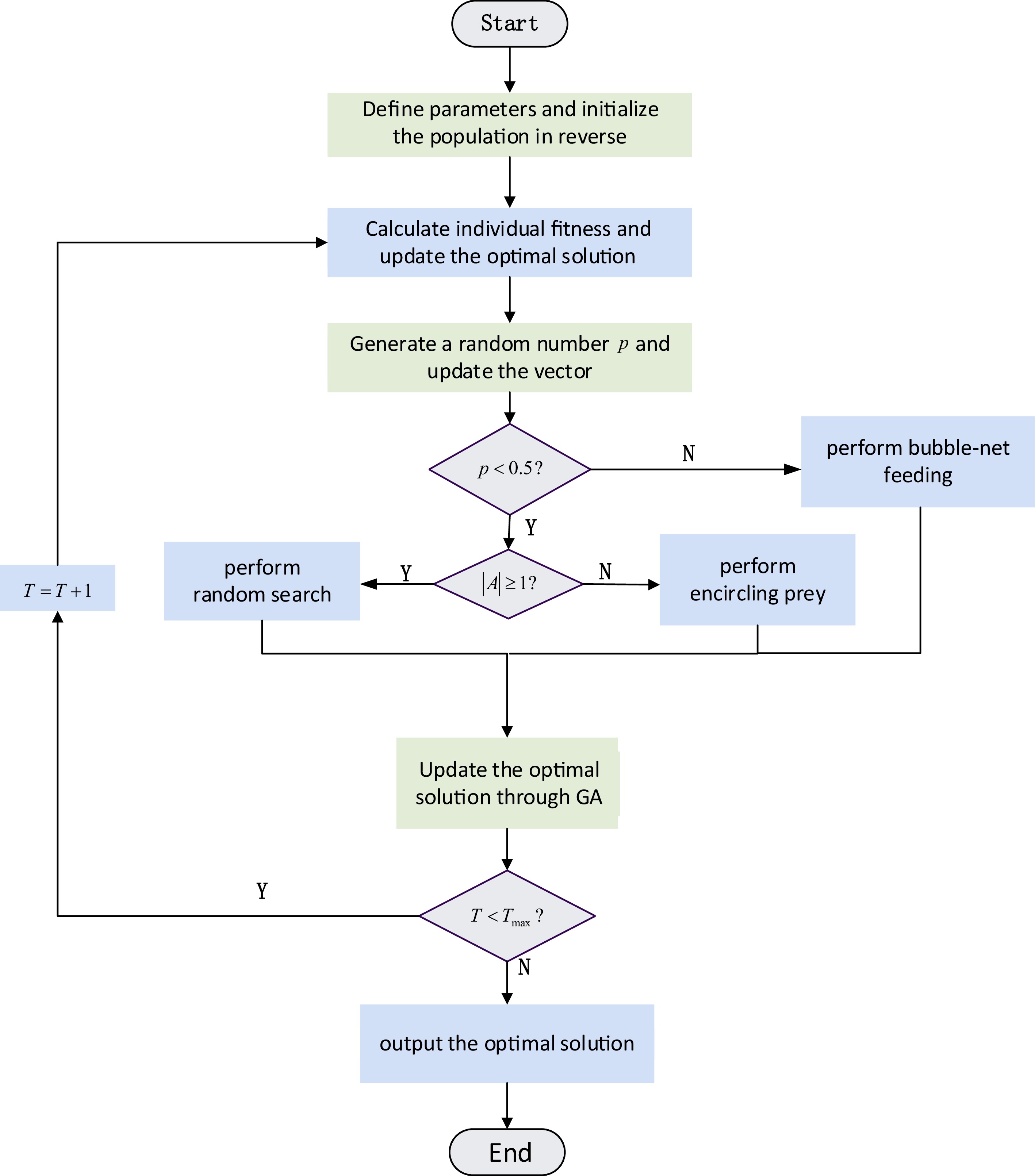
Figure 3. 

Flow chart of IWOA. The modules marked in green correspond to the improvement mechanism, while the remaining modules follow the standard WOA process.

Backward learning mechanism

During population initialization, the reverse-learning mechanism generates initial populations with broader distributions and higher quality. Simultaneously, it evaluates both random solutions and their reverse counterparts within the solution space, selecting the optimal configuration. This effectively prevents premature convergence stagnation caused by errors arising from blind initialization^[23,24]. The reverse learning initialization can be expressed by Eqs (16) and (17):

Where, $ p $ denotes the $ p $^th individual in the population, $ d $ represents the $ d $^th dimension in space, $ u $ and $ e $ denote the upper and lower bounds of the search space, respectively, $ X $ is the initial population, $ {x}_{pd} $ is the individual population, $ {X}^{\prime} $ is the inverse solution of the population, $ {x}_{pd} $ is each individual in the initial population, $ x_{pd}^{\prime} $ is the back-propagation learning factor, and $ {l}_{sca} $ denotes the random scaling coefficient, whose random value lies between $ \left[0,2\right] $.

Nonlinear convergence factor

The original linear convergence factor has been replaced by a non-linear decay strategy characterized by early slowness and late rapidity. This approach allocates extended global exploration time during the algorithm's initial stages to uncover potential optimal regions, subsequently shifting rapidly to refined local exploitation in later phases. This achieves an excellent dynamic equilibrium between exploration and exploitation. The proposed enhanced WOA algorithm employs a nonlinear convergence factor to replace the following specific Eq. (18):

Among these, $ \varepsilon =1 $, $ \beta =0.5 $, $ \gamma =50 $.

Random number generation mechanism

Whilst retaining the inherent random decision mechanism of WOA^[25], additional random factors were introduced during stages such as the reverse learning phase. This enhances the algorithm's capacity to generate diverse solutions during iteration, significantly improving its robustness in escaping local optimum traps.

Based on genetic algorithms (GA)

To mitigate the premature convergence and local stagnation issues encountered by the standard WOA in complex, high-dimensional search spaces, this paper incorporates GA operators into the iterative process. The core of GA lies in crossover and mutation, generating offspring, and exploring the solution space to discover superior solutions. In this study, new solutions are generated by comparing the current solution with another solution produced through crossover and mutation, then selecting the superior solution as the optimal solution for the current generation. Crossover simulates the exchange of genetic information between two individuals. The corresponding expressions are given in Eqs (19) and (20):

where, $ {g}_{1} $ and $ {g}_{2} $ represent the parent individuals, $ {g}_{new} $ denotes the offspring individual, $ \beta $is the crossover coefficient, $ \mu {}_{i}\sim U\left(0,1\right) $is the crossover control parameter, and $ \eta $ is a binary variable $ {r}_{i}\in \left\{0,1\right\} $, used to control crossover directionality. This paper introduces GA-based recombination and mutation operations, periodically generating promising candidate solutions around elite individuals. This approach preserves WOA's exploration capability while injecting structured diversity, thereby enhancing the ability to escape local optima and improving final convergence accuracy.

Improved Adaptive Large-Scale Network Simulation (IALNS)

The ALNS algorithm^[26] has been extensively applied to complex combinatorial optimization problems. Its core principle involves evolving solutions through iterative destroy-and-repair operations. Traditional ALNS generates an initial solution and treats it as the current optimum. During iteration, new solutions are produced through destruction and repair operations, with acceptance governed by a roulette wheel mechanism until the maximum iteration count is reached, or other termination criteria are satisfied. However, such initialization is prone to becoming trapped in local optima, from which escape proves difficult. Furthermore, the lack of adaptability in operator selection and weight adjustment mechanisms leads to computational inefficiency, particularly when handling large-scale problems. To address these issues, this study employs a K-means clustering strategy^[27] during the algorithm's initialization phase. During the solution update phase, simulated annealing is utilized to determine whether new solutions should be accepted within the IALNS framework. The algorithmic workflow is illustrated in Fig. 4.

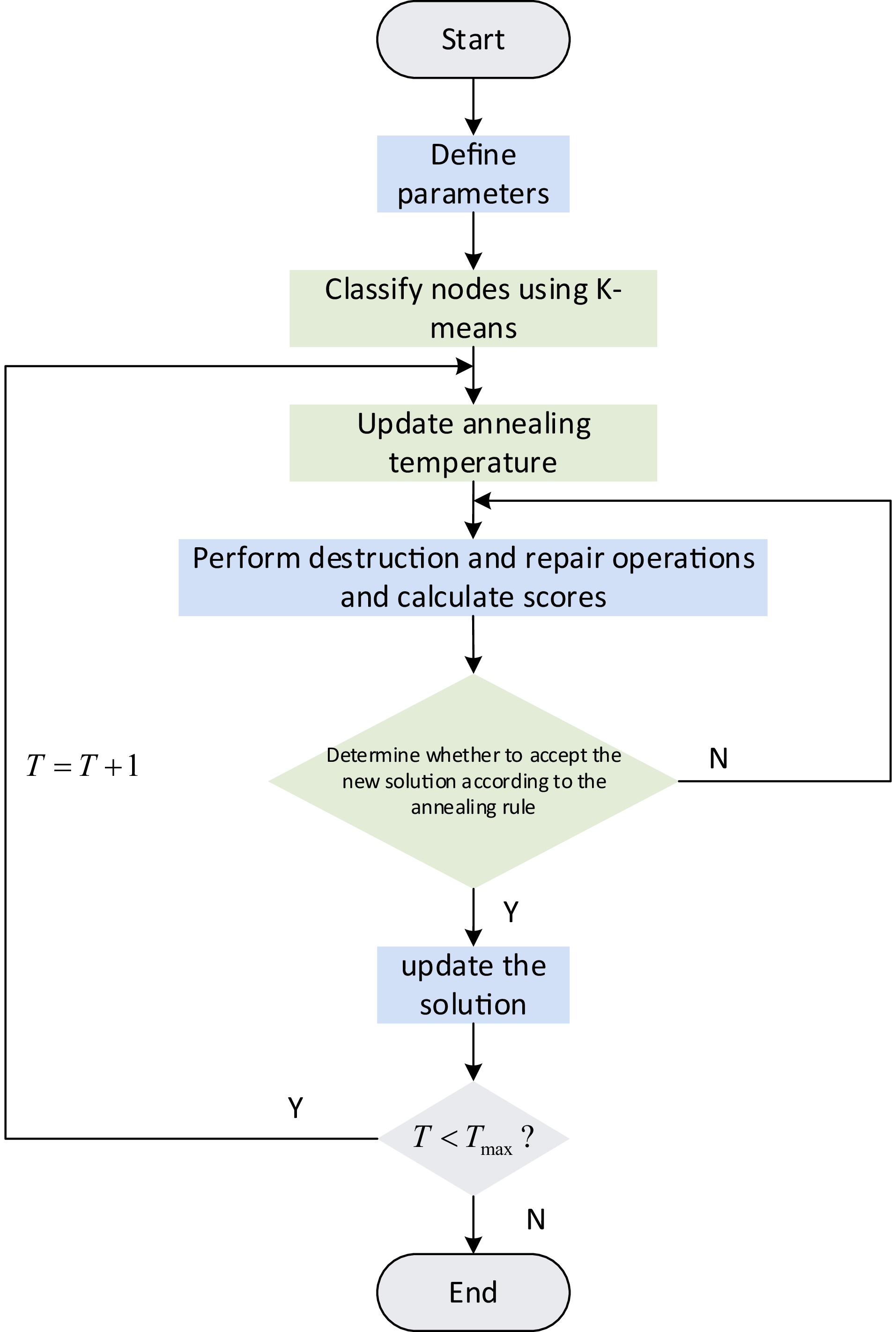
Figure 4. 

Flowchart of IALNS. The modules marked in green correspond to the improvement mechanism, while the remaining modules follow the standard ALNS process.

K-means clustering

The K-means clustering method partitions a given dataset into distinct clusters, such that data points within the same cluster exhibit high similarity, while those across different clusters display relatively low similarity. Its core principle involves iteratively searching for cluster centers to minimize the sum of distances between each data point and its assigned cluster center. In this study, the number of clusters equates to the number of deployed drones. The clustering formula for K-means is presented in Eq. (21):

Simulated annealing mechanism

Simulated annealing (SA) is a general-purpose probabilistic algorithm frequently employed to locate global optima within extensive solution spaces^[28]. Its core principle lies in the acceptance criterion, defined by Eq. (22):

where, $ {P}_{acp} $ denotes the probability of accepting a new proposal, $ \nabla f $ represents the difference between the objective function values of the new proposal and the current solution, and $ T $ indicates the current temperature. The ALNS algorithm is prone to becoming trapped in local optima during the search process. To address this issue, IALNS incorporates the concept of simulated annealing, permitting the algorithm to probabilistically accept suboptimal solutions under specific conditions. This facilitates escape from local optima, expands the search space, and increases the likelihood of discovering the global optimum.

This study employs simulation experiments conducted on the MATLAB R2024a platform, utilizing the underlying research framework for site selection and flight path planning, with data subsequently transmitted to the top-level layer for task allocation. To ensure the reliability of experimental results and their practical applicability, this study strictly adheres to the UAV performance parameters outlined in Table 3 when randomly generating 10 task points. Notably, the settings for maximum payload, safe altitude, and cruising speed directly determine the calculation of cost terms within the LRSP model and the feasibility of task allocation by the IALNS algorithm. At the same time, to ensure the scalability of the model, the experiments will be divided into two types: lightweight experiments, and complex experiments. The lightweight scene experiment includes 10 task points, while the complex experiments will include 20 task points. All task point information is shown in Table 3:

To reflect real-world conditions, this study also defined performance parameters for the UAV as shown in Table 4.

Experimental results

Lightweight scene experiment

First, the IWOA algorithm and the WOA algorithm successfully determined the optimal location for the central distribution center within the underlying model. As illustrated in Fig. 5, the final coordinates of the distribution center were determined to be (206.32, 303.84, 48.11) under the iterations of both algorithms. This result demonstrates that the site-selection objective function can form a stable global optimum within the feasible region. This location effectively balances the average service distance to all task points while avoiding high-risk terrain areas. It demonstrates the advantage of jointly modelling average service distance and terrain elevation penalties within the site selection model, providing an efficient starting point for subsequent path planning and task allocation.

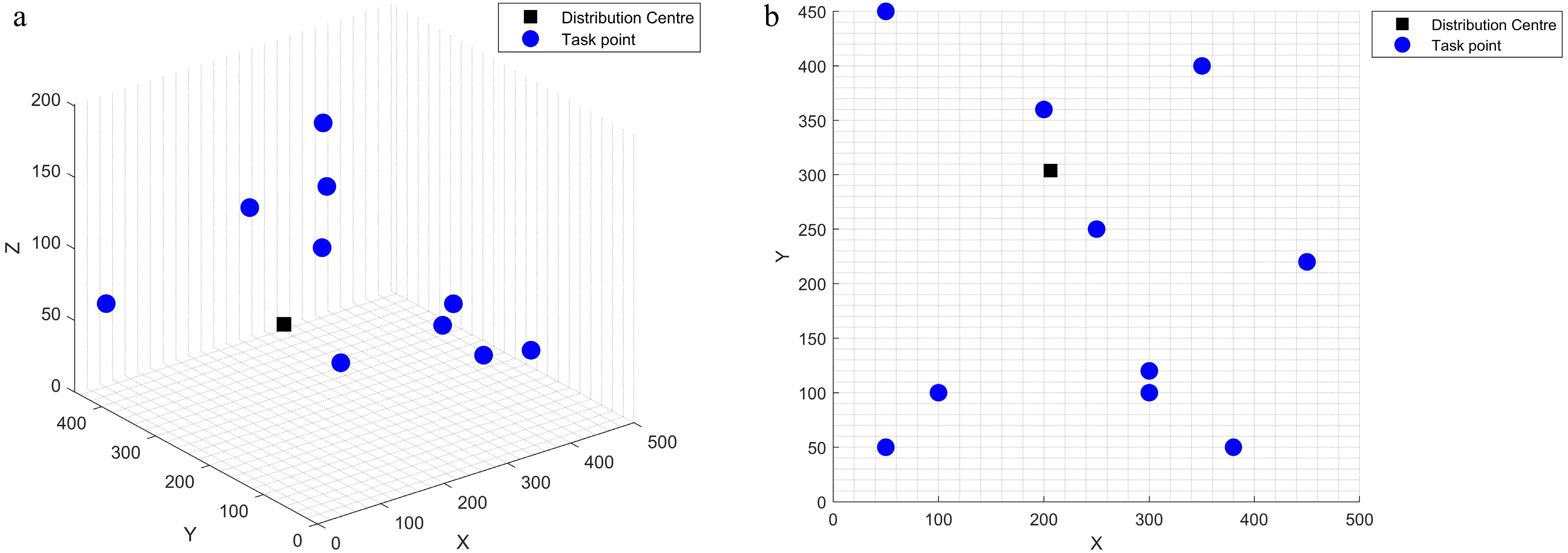
Figure 5. 

Hub location schematic. (a) Side view of spatial distribution. (b) Top view of spatial distribution.

Following the determination of the distribution center's location, the top-level algorithm performed multi-UAV collaborative task allocation and scheduling for 10 mission points based on the trajectory cost matrix generated at the lower level. Table 5 presents the final mission execution results.

Table 5 summarizes the performance differences between the two generation algorithms under identical workload distribution conditions. For the WOA–ALNS algorithm, the total flight distance was 3,155.4022 km, with an average flight distance per drone of 1,051.8007 km. In contrast, the IWOA–IALNS algorithm achieved a total flight distance of 2,885.0083 km, with an average flight distance per drone of 961.6694 km. The model-solving framework formed by the improved algorithm reduced the total flight distance by 270.3939 km, representing an improvement of 8.57%. Additionally, the maximum single-trip distance decreased from 1,645.1407 km to 1405.1481 km—a reduction of 239.9926 km (14.59%). This alleviates long-distance task allocation in worst-case scenarios, enhancing feasibility within time window and endurance constraints.

The planned trajectories are shown in Figs 6, 7.

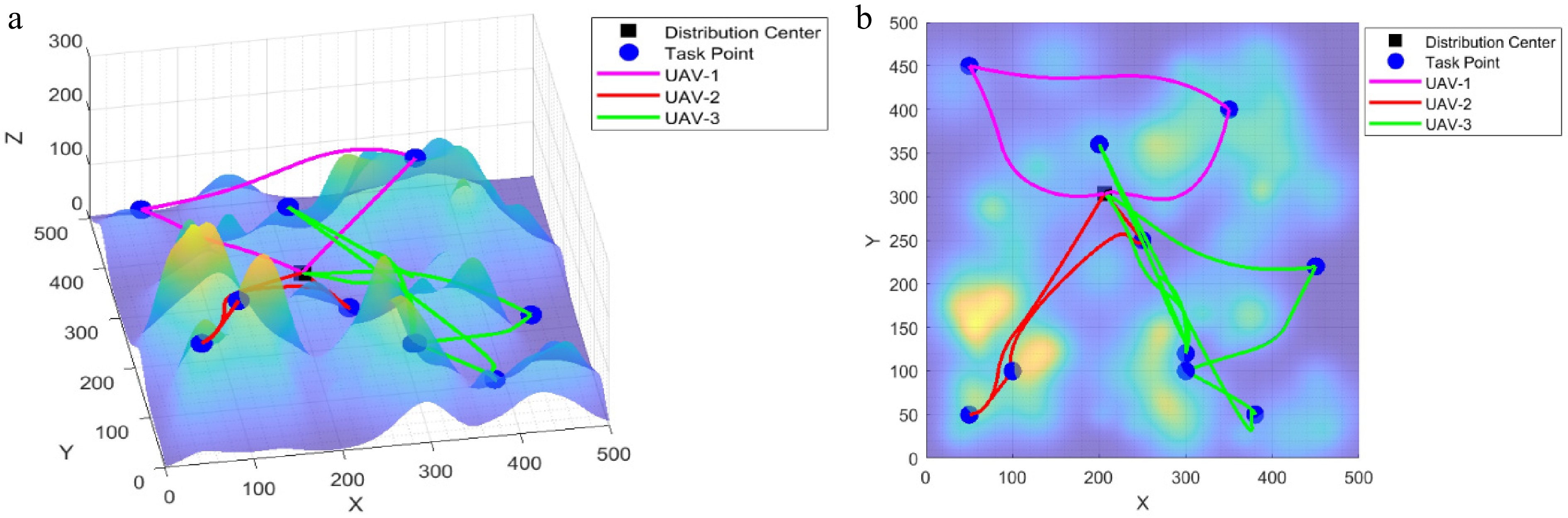
Figure 6. 

Planned trajectory diagram of WOA–ALNS; (a) side view, and (b) top view.

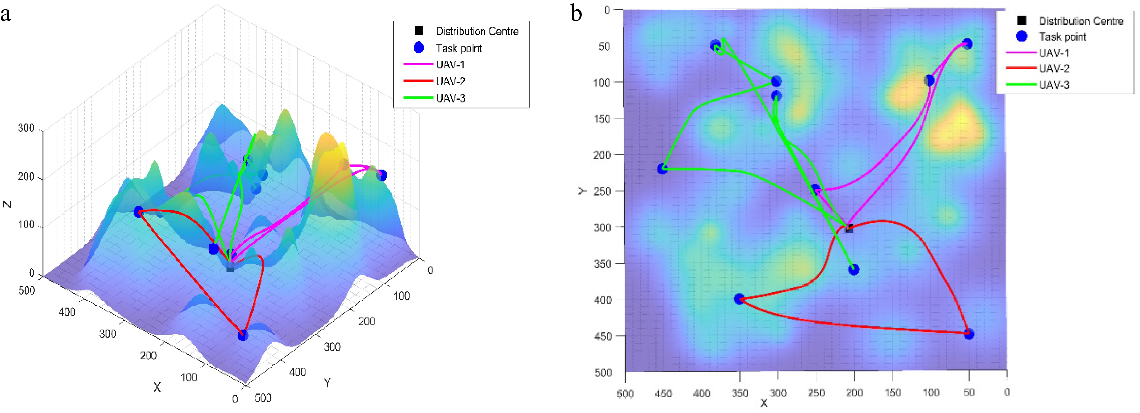
Figure 7. 

Planned trajectory diagram of IWOA–IALNS; (a) side view, and (b) top view.

These flight paths illustrate the optimized three-dimensional trajectories produced under the two-layer LRSP framework for the 10-task-point light scenario. In both models, the lower-layer path planner generates feasible routes by explicitly considering terrain clearance, no-fly-zone avoidance, and altitude-related costs, and the resulting trajectory cost matrix is then provided to the upper-layer scheduler to determine the task sequence and hub-returning tours. As shown in Fig. 6, all three drone routes can complete all assigned tasks through hub-and-spoke return-to-base cruising. However, the top view reveals that Route 3's path is complex. In the side view, the corresponding trajectory repeatedly traverses rugged terrain, incurring higher altitude penalties in complex topography. Figure 7 presents a top-down view where the mission routes better align with spatial clustering characteristics, significantly reducing long-distance traversals between remote areas. The side-view trajectory appears smoother and more terrain-contouring, indicating that the underlying trajectory cost construction provides the upper-layer scheduler with more informative boundary costs.

Complex scene experiment

To further evaluate the scalability and robustness of the proposed two-layer LRSP framework in large-scale scenarios, this section constructs a complex scenario comprising 20 task points. Compared to the 10-task-point case, this scenario exhibits higher combinatorial complexity in task sequencing and UAV allocation, presenting more severe feasibility challenges under mountainous terrain constraints and no-fly zone restrictions. The coordinates, workload requirements, and time windows for the 20 task points are summarized in Table 2. To ensure fairness, drone parameters and cost-related settings follow the configurations in Table 3. Both algorithmic models were run under identical termination conditions and computational budgets, including population size, maximum iterations, and stopping thresholds. First, both algorithms yield the distribution center coordinates as (267.96, 256.11, 23.34). The pivotal position is shown in Fig. 8.

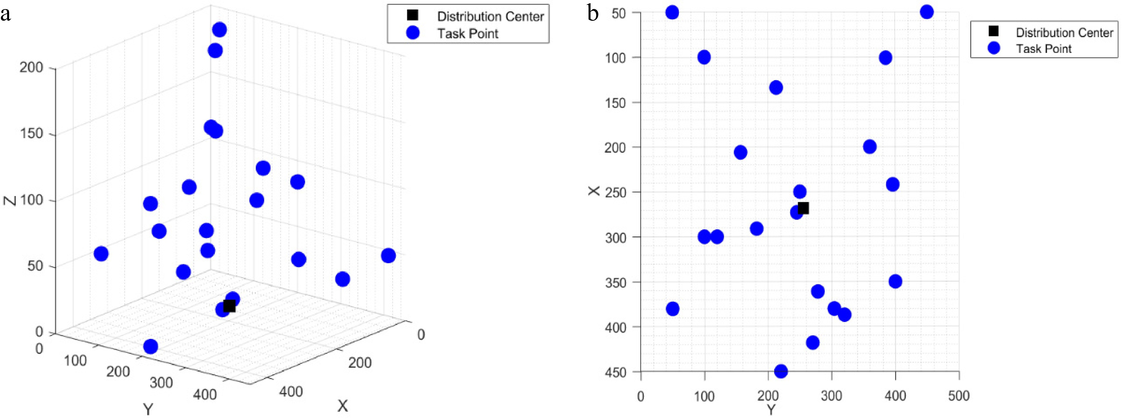
Figure 8. 

Hub location schematic; (a) side view of spatial distribution, and (b) top view of spatial distribution.

Table 6 shows the final task execution results of the two algorithms.

Table 6 presents the task execution statistics for the two algorithmic models. In the scenario with 20 task points, both WOA–ALNS and IWOA–IALNS deployed six drones to complete all delivery tasks, with identical total workloads across both schemes, indicating the comparison was conducted under equivalent service demand levels.

The WOA–ALNS scheme generated a total flight distance of 3,932.6480 km, with an average flight distance per drone of 655.4413 km. Notably, the longest route reached 1,227.3709 km, indicating the algorithm framework's tendency to generate highly elongated routes for individual drones, potentially increasing operational risks and time window pressures. In contrast, the proposed IWOA–IALNS achieved a total flight distance of 3,439.6351 km, reducing the average flight distance per drone to 573.2725 km. Compared to WOA–ALNS, the total distance decreased by 493.0129 km, equivalent to a 12.54% reduction in overall flight distance. Furthermore, the maximum single-trip distance decreased from 1,227.3709 to 859.4272 km, a reduction of 29.98%, indicating that IWOA–IALNS effectively mitigates the assignment of extremely long-distance tasks, and constructs a more operationally feasible flight route structure.

From a workload distribution perspective, although the average workload and total workload were identical for both methods, IWOA–IALNS exhibited lower workload dispersion: the standard deviation decreased from 7.64 to 6.45, representing an improvement of approximately 15.48%. This indicates more balanced task distribution among UAVs.

The flight path planning is shown in Figs 9, 10.

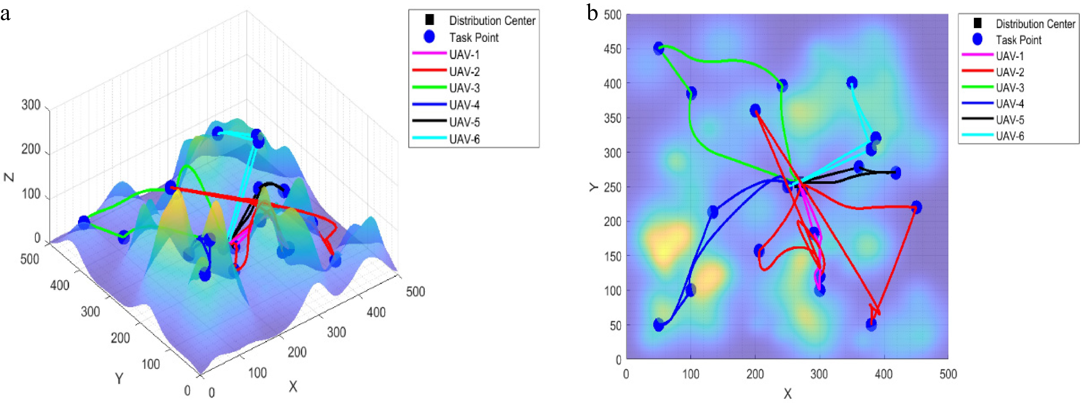
Figure 9. 

Planned trajectory diagram of WOA–ALNS; (a) side view, and (b) top view.

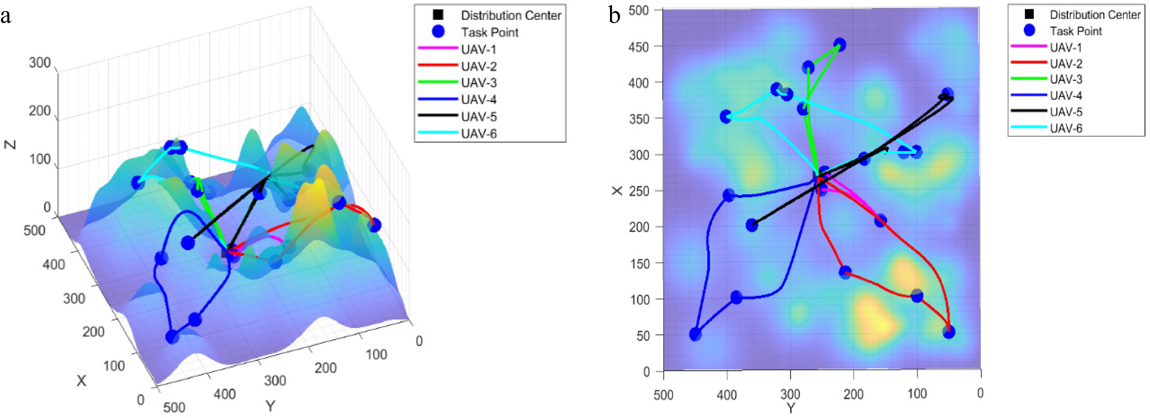
Figure 10. 

Planned trajectory diagram of IWOA–IALNS; (a) side view, and (b) top view.

As shown in Fig. 9, although all drone routes originate and terminate at the distribution center, several trajectories exhibit long-distance cross-regional traversals and significant route folding and stretching in the plan view. This indicates that the baseline scheme tends to generate elongated routes spanning dispersed task clusters. In the side view, routes adjust altitude more frequently over elevated terrain, potentially accumulating higher altitude costs during mountainous operations. Figure 10 presents a more structured and compact path pattern. In the top view, task points are covered by routes more aligned with cluster characteristics, with a marked reduction in long-distance traversals between remote areas. This indicates improved spatial task partitioning among UAVs. The side view shows smoother terrain contouring, suggesting that the underlying path planning and trajectory cost matrix provide more valuable cost information to the upper-layer scheduler. This facilitates more efficient task allocation and sequencing decisions.

The four experimental cases in simulation experiment collectively verify that the proposed dual-layer LRSP framework for mountainous UAV logistics exhibits strong effectiveness and scalability. Across all experiments, the lower-layer planner is able to generate feasible three-dimensional flight trajectories that satisfy terrain-clearance and no-fly-zone avoidance constraints, and feeds the resulting trajectory costs back to the upper layer via a trajectory cost matrix. When the problem scale is expanded from 10 task points to 20 task points, the framework still maintains feasibility and produces a stable integrated solution system covering hub location selection, routing, and task servicing. The proposed IWOA–IALNS model consistently outperforms the baseline WOA–ALNS. The improvements are reflected not only in reduced total flight distance and shortened maximum route length, but also in more balanced UAV workload allocation and more reasonable spatial partitioning of task points. Moreover, the superiority of IWOA–IALNS becomes more pronounced in the complex scenario, demonstrating the proposed framework's strong adaptability to more challenging instances.

This paper addresses the planning and optimization challenges of unmanned aerial vehicle (UAV) logistics networks within mountainous transportation systems by proposing a two-layer collaborative optimization model for location selection and flight path planning-task assignment (LRSP). The model aims to unify decision-making for distribution center siting, three-dimensional flight path planning, and multi-UAV task allocation, thereby minimizing overall system transportation costs. The lower layer implements three-dimensional flight path planning within complex terrain, while the upper layer handles dynamic multi-UAV task allocation and scheduling. Information exchange and cost feedback between layers occur via a trajectory matrix, enabling unified decision-making for trajectory generation and task scheduling within the logistics system.

Simulation results show that in the lightweight 10-task-point experiment, both models use the same number of UAVs and satisfy identical workload requirements; however, IWOA–IALNS reduces the total flight distance from 3,155.4022 to 2,885.0083, achieving an 8.57% reduction. Meanwhile, it decreases the maximum single-route distance from 1,645.1407 to 1,405.1481, corresponding to a 14.59% reduction, thereby alleviating the worst-case long-haul assignment. In the complex 20-task-point experiment, the proposed method exhibits a more pronounced advantage: the total flight distance is reduced from 3,932.6480 to 3,439.6351, i.e., a 12.54% reduction, and the maximum single-route distance decreases from 1,227.3709 to 859.4272, i.e., a 29.98% reduction. Meanwhile, workload allocation becomes more balanced, with the standard deviation of workloads decreasing from 7.64 to 6.45, indicating improved scheduling stability. The improved algorithm demonstrates enhanced model robustness and successfully completes distribution center site selection and multi-UAV collaborative operations in typical mountainous terrain, ensuring both flight path feasibility and safety. This study not only validates the effectiveness of the dual-layer collaborative optimization framework, but also provides an extensible intelligent optimization method for drone logistics network planning in low-altitude economic environments. Future research may explore dynamic environment modeling, multi-center collaborative optimization, integrated energy consumption-load modeling, and intelligent learning algorithm fusion. These advancements will drive the development of smarter, adaptive, and real-time responsive drone logistics dispatch systems, accelerating the digital and intelligent evolution of low-altitude transportation systems.