A satellite-MAV cooperative regional imaging method based on grey wolf optimization and multi-base MAVs fast path planning

Figure 1 presents a schematic diagram of satellite-MAV cooperative observation. As ground search and regional observation tasks increasingly demand larger scale, higher timeliness, and higher precision, a single platform often struggles to simultaneously guarantee search efficiency, coverage completeness, and fast task response under complex mission conditions. Agile satellites offer advantages such as large coverage area, high observation speed, and the ability to perform side-swing maneuver imaging, enabling large-scale regional search within a relatively short time. However, limited by constraints such as imaging swath width, side-swing angle limitations, and orbital conditions, satellite coverage over complex regions may still suffer from edge omissions, local blind spots, or residual gaps between adjacent strips. In contrast, MAVs feature flexible deployment, high maneuverability, and strong local fine-search capabilities, allowing them to rapidly conduct supplementary searches in the uncovered areas left by satellites. Therefore, investigating the mission planning problem for agile satellite-MAV cooperative search is of great significance for improving regional search efficiency and resource utilization efficiency in complex scenarios.

Figure 1. 

Schematic diagram of satellite-MAV cooperative observation.

Extensive studies have been conducted on MAV coverage path planning, multi-MAV cooperative scheduling, space-air-ground collaborative observation, and intelligent optimization algorithms, laying an important foundation for complex regional search tasks. In terms of multi-platform collaborative observation, relevant studies have shown that satellites, MAVs, and ground observation platforms exhibit significant complementarity in observation range, resolution, and response speed. Lei et al. integrated satellite imagery, MAV aerial photography, and ground observations to construct a space-air-ground integrated flood disaster monitoring and assessment system, pointing out that satellite remote sensing is suitable for large-scale disaster monitoring, while MAVs and ground observations are better suited for localized refined emergency assessment^[1]. Li et al. obtained parameters of the local motion and long-distance transport of river ice through combined MAV and GPS observations, demonstrating that air-ground cooperative observation can compensate for the limitations of a single platform in terms of spatial coverage and continuous tracking capability^[2]. Furthermore, Wang et al. investigated the coordination mechanism between satellites and MAV nodes from the perspective of multi-agent task scheduling in space-air-ground integrated networks^[3]. Khatiwoda et al. and Abdel-Basset et al., respectively, validated the application potential of space-air-ground collaborative systems from the perspectives of MAVs, low-orbit satellites, and non-terrestrial network coverage optimization^[4,5]. These studies confirm that multi-platform collaboration can effectively enhance observation capabilities in complex areas. However, most existing studies focus on system construction, communication coverage, or data acquisition, while the problem of task allocation and path planning for MAVs to perform supplementary searches after satellite imaging coverage remains relatively underexplored.

In terms of MAV coverage search and path planning, a relatively mature methodological framework has been established in existing studies. Yu et al. proposed a multi-base multi-MAV cooperative coverage path planning algorithm for complex area coverage missions considering flight time, energy constraints, and multi-base takeoff and landing conditions. The robustness of the algorithm was validated through comparison with traditional sweep-based coverage methods^[6]. Although such studies are relevant to the multi-base MAV supplementary search problem addressed in this paper, they typically plan full-area coverage paths rather than dynamically generating supplementary paths based on remaining grids after satellite coverage. Yang et al. proposed an online coverage path planning method integrating Boustrophedon motion and the D* algorithm for unknown area mapping missions^[7]. Caballero et al. modeled multi-MAV inspection tasks as a capacitated multi-depot vehicle routing problem^[8]. Chou et al. investigated task allocation and path planning from the perspective of MAV-assisted Internet of Things data collection^[9]. Furthermore, Nafees et al. systematically reviewed the algorithmic workflows, optimization models, and challenges in MAV path planning, noting that real-time performance, multi-MAV coordination, energy constraints, and environmental uncertainty remain important issues in this field^[10].

For MAV local navigation, obstacle avoidance, and trajectory optimization in complex environments, existing studies mainly focus on perception and mapping, model predictive control, and trajectory smoothing. Lindqvist et al. and Wang et al. investigated MAV navigation and trajectory optimization methods based on reactive obstacle avoidance constraints and octree adaptive resolution, respectively^[11,12]. Guo et al. investigated the time-coordinated trajectory planning problem in MAV formation flight^[13]. Furthermore, Hattenberger et al. discussed the influence of environmental factors on MAV path planning from the perspective of wind field estimation^[14]. These studies focus on local obstacle avoidance, trajectory generation, or environmental adaptation, whereas this paper focuses on the global coupling optimization between satellite coverage strategies and MAVs' supplementary search costs.

Multi-base multi-MAV task allocation and path optimization are also important research directions in this field. Ahmadi et al.^[15], Wen et al.^[16], and Li et al.^[17] investigated multi-depot MAV delivery, bi-level programming for multi-depot multi-MAV systems, and multi-base path planning under uncertain flight time conditions, respectively. Zhao et al.^[18] and Peng et al.^[19] further discussed multi-platform collaborative path optimization from the perspectives of dynamic multi-MAV path planning under uncertain environments and electric vehicle-MAV collaborative delivery. These studies indicate that multi-base path planning typically involves complex constraints and high combinatorial optimization complexity; however, their mission backgrounds mainly focus on delivery, inspection, or data collection, which still differ from the supplementary search of remaining grids in satellite-MAV collaborative area imaging.

In terms of intelligent optimization algorithms, methods such as grey wolf optimization, genetic algorithms, particle swarm optimization, simulated annealing, and deep reinforcement learning have been widely applied to MAV path planning and cooperative scheduling. Zhang et al. proposed an improved grey wolf optimization algorithm integrating Lévy flight and multi-population mechanisms to solve the energy-efficient cooperative path planning problem of multiple MAVs, to improve the algorithm's ability to escape local optima^[20]. Jamshidi et al.^[21], Geng et al.^[22], and Sun et al.^[23] improved the grey wolf optimization algorithm from the perspectives of parallel computing, chaotic initialization, and multi-population updating, and applied it to three-dimensional MAV path planning or multi-MAV trajectory planning. Furthermore, Xu et al.^[24], Chen et al.^[25], and Zhang et al.^[26] investigated MAV path planning problems using multi-strategy fusion optimization algorithms, starling swarm bionic algorithms, and LSTM-based deep reinforcement learning methods, respectively. Wang et al.^[27] and Xun et al.^[28] demonstrated the application potential of deep reinforcement learning and hierarchical optimization methods in the joint optimization of MAV trajectory planning and task offloading. These studies indicate that intelligent optimization algorithms are highly adaptable to complex path planning problems; however, few studies have integrated satellite side-swing coverage strategies and MAV supplementary path costs into a unified optimization framework.

In addition to MAV path planning, intelligent optimization methods have also been applied to satellite selection and space-air-ground resource optimization. Dai et al. proposed a fast satellite selection method based on a non-dominated sorting whale optimization algorithm and compared it with grey wolf optimization, particle swarm optimization, and genetic algorithms^[29]. Chang et al. proposed a dual-MAV cooperative localization system, demonstrating the application value of multi-MAV cooperative sensing in target localization tasks^[30].

In summary, existing research has made considerable progress in MAV coverage path planning, multi-base path optimization, space-air-ground collaborative observation, and the application of intelligent optimization algorithms. However, for agile satellite and MAVs collaborative area imaging missions, the following research gaps remain. First, most existing studies focus on the independent optimization of either satellites or MAVs as single platforms, with insufficient consideration of the coupling relationship between large-area satellite coverage and local MAVs' supplementary search. Second, existing MAV coverage path planning typically directly plans paths for the entire mission area and rarely involves rapid supplementary path generation for discrete remaining grids after satellite coverage. Third, the reverse impact of multiple bases, range constraints, and supplementary search costs on satellite side-swing strategies has not been fully considered. Fourth, although intelligent algorithms such as grey wolf optimization have been applied to MAV path planning, further research is still needed on side-swing angle optimization, boundary processing, and fitness construction for cooperative coverage in satellite-MAV collaborative area imaging tasks.

To address the above issues, this paper investigates the agile satellite and MAV cooperative search mission and proposes a satellite-MAV collaborative area imaging method based on grey wolf optimization and multi-base MAV fast path planning (GW-SWCRI). A unified framework for satellite-MAV collaborative area coverage and supplementary search planning is established. On this basis, the satellite side-swing angle is adopted as the optimization encoding object, and a fitness function that comprehensively considers the MAVs' supplementary search cost and the satellite attitude adjustment cost is established. An improved grey wolf optimization algorithm is employed to perform a global search for satellite coverage strategies. For the remaining grids after satellite coverage, a multi-base MAV fast path planning method is proposed to achieve fast partitioning and path generation of the supplementary search area under range constraints. Finally, simulation experiments under different mission scenarios are conducted to validate the effectiveness, stability, and scenario adaptability of the proposed method.

To support rapid wide-area imaging and supplementary observation, this paper establishes a unified planning model for collaborative area imaging by agile satellites and MAVs. All MAVs discussed in this paper refer to micro fixed-wing unmanned aerial vehicles. Given the substantial differences in mission objectives, platform capabilities, and operational constraints between satellite coverage and MAVs' supplementary imaging, collaborative planning must account for both the pre-coverage performance of satellite pushbroom imaging over the target area and the distribution of MAVs' takeoff bases, local maneuverability, and individual range constraints, to enable rapid supplementary imaging of remaining uncovered areas. Therefore, based on a gridded representation of the mission area, this paper establishes a satellite coverage model and an MAV supplementary imaging model, and integrates both within a unified collaborative planning framework.

Within this framework, the satellite first conducts area pushbroom imaging under a given side-swing angle scheme during its visible time window, producing initial coverage results for the mission area. Subsequently, the remaining grids not fully covered by the satellite serve as the input for MAVs' mission planning, and multi-base MAVs carry out supplementary imaging. Since MAVs can only image at the centers of discrete grids and each waypoint covers multiple adjacent grids, this task is essentially a combinatorial optimization problem involving coverage determination, waypoint selection, base assignment, path sequencing, and range constraints. To clarify the subsequent modeling and algorithm design, this chapter systematically formulates the satellite-MAV collaborative planning problem in terms of model constraints, mission area discretization, satellite and MAV models, operational framework, and fitness function design.

Model constraints

To ensure the feasibility of the satellite-MAV collaborative area imaging mission and the rigor of model formulation, this paper defines the following basic constraints for the satellite-MAV collaborative planning problem in the modeling stage:

(1) The mission area is discretized into regular grids. Any grid that is effectively covered once is considered fully covered, and repeated coverage is not counted toward the coverage benefit.

(2) The satellite first performs area pushbroom imaging. Grids that are fully covered by the satellite are no longer assigned to MAVs; grids that are only partially covered are still regarded as targets requiring supplementary imaging.

(3) MAVs are only allowed to perform imaging operations at the centers of discrete grids, and path planning is conducted on the set of grid centers corresponding to candidate waypoints.

(4) Each selected waypoint is visited exactly once and assigned to one MAV flight path to avoid repeated visits.

(5) Any grid requiring supplementary imaging only needs to be effectively covered once by a single MAV; once this grid has been covered, it will be removed from the pending task set.

(6) Each MAV path starts from a designated takeoff base, and each path is associated with exactly one takeoff base; MAVs from different bases jointly complete the supplementary imaging task for the remaining area.

(7) The total flight distance of any MAV flight path shall not exceed the maximum range of a single MAV. The maximum range mentioned in this paper includes reserved return-flight redundancy. Therefore, no separate return segment is added during path construction.

Satellite-MAV collaborative problem model

Mission area discretization

Discretizing the target imaging area into regular grids enables more intuitive evaluation of coverage provided by satellites and MAVs. The mission area is discretized into a set of regular grids as follows:

where $ {g}_{x,y} $ denotes a grid with horizontal and vertical coordinates $ (x,y) $, respectively. Each grid is associated with a unique center point, which is defined as:

where $ {\lambda }_{x,y} $ and $ {\phi }_{x,y} $ represent the longitude and latitude of the grid center point, respectively. The grid has two possible states during mission planning, namely covered and uncovered, which are defined as:

where $ {g}_{\mathrm{cov}} $ indicates that the grid is marked as covered, and $ {g}_{unc} $ indicates that the grid is marked as uncovered. $ Sa{t}_{Cover} $ denotes that the satellite swath fully covers $ {g}_{x,y} $; $ MA{V}_{Image} $ denotes that the MAV has already imaged $ {g}_{x,y} $; $ Sa{t}_{Cross} $ denotes that the satellite swath only partially covers $ {g}_{x,y} $. Thus, for the $ Sa{t}_{Cross} $ state, grids are defaulted to require supplementary imaging by the MAV. After determining the satellite coverage status, $ g_{x,y}^{res} $ is obtained and used as the input for MAV path planning.

Note that the target area is discretized using fixed longitude and latitude intervals. Although grids with uniform geographic spacing have varying ground footprint areas at different latitudes, especially in the longitudinal direction, these differences are negligible in this work, as the target region spans a limited latitudinal range. Furthermore, the grid resolution is determined based on the swath widths of both satellites and MAVs. Thus, each grid cell serves as the fundamental unit for coverage evaluation and path planning. Grid cells with only partial coverage are classified as incompletely covered and require supplementary imaging by MAVs.

Satellite model

The satellite model takes a single satellite as an input parameter. The set of satellites visible to the target area within the mission time window is defined as:

where $ N $ denotes the total number of satellites available for the mission. The attributes of a single satellite are defined as:

where $ Vi{s}_{ST} $ and $ Vi{s}_{ET} $ are the visible start time and visible end time of the satellite $ Sa{t}_{i} $ for the imaging target, respectively. $ ecef_{i}^{X} $ and $ ecef_{i}^{V} $ are the position and velocity of $ Sa{t}_{i} $ in the Earth-centered Earth-fixed coordinate system during the interval $ [Vi{s}_{ST},Vi{s}_{ET}] $, respectively. $ Att_{i}^{\min } $ and $ Att_{i}^{\max } $ are the lower and upper bounds of the side-swing angle of $ Sa{t}_{i} $, respectively. $ {W}_{i} $ is the imaging swath width of $ Sa{t}_{i} $.

MAV model

Base set and MAV mission mode

This section addresses the complete path planning of MAVs departing from their bases to observation waypoints. Multiple MAV bases are deployed around the mission area, and the set of bases is defined as:

Each base $ {B}_{m} $ corresponds to a grid center coordinate. Each MAV takes off from a designated base and sequentially visits target grids to complete the imaging task. A flight path of an MAV is defined as:

where $ {B}_{m} $ denotes the takeoff base of the MAV, and $ {v}_{xi,yi} $ denotes the $ i $-th waypoint along the flight path, which corresponds to the grid center $ {p}_{xi,yi} $ of grid $ {g}_{xi,yi} $.

Cross-shaped imaging coverage model

Given the attitude adjustment range and the imaging characteristics of the mission payload, the MAV can only perform imaging at grid center points. When the MAV is positioned at $ {g}_{x,y} $, the set of grids it covers is:

where $ C(x,y) $ denotes the set of grids covered when the MAV is located at $ {g}_{x,y} $, including the grid itself and its adjacent grids. Grids outside the area boundary are excluded from the coverage calculation.

Distance calculation model

Calculating flight distances between grids using only longitude and latitude coordinates can introduce significant errors. This paper adopts the Haversine formula to calculate the distance between two grids. For two grid centers $ {p}_{i} $ and $ {p}_{j} $, the spherical distance is given by:

where $ R $ is the mean Earth radius. All path lengths, base-to-waypoint distances, and flight distances between grid centers in this paper are calculated using this formula.

Range constraints and mission time

For a given flight path, its total flight distance and corresponding constraints are defined as :

where $ {D}_{\max } $ denotes the maximum range constraint of the MAVs.

Model operation framework

To achieve collaborative optimization between agile satellites and MAVs in area imaging missions, this paper develops an operational framework, as shown in Fig. 2. The framework consists of four sequentially connected functional layers: input layer, modeling layer, optimization layer, and output layer. The input layer imports basic parameters including the target region, constellation settings, and MAV flight range constraints; the modeling layer performs task region discretization and satellite visibility preprocessing. As the core module, the optimization layer follows the sequence of GWO-based side-swing angle optimization, satellite coverage calculation, remaining uncovered grid extraction, multi-base MAV fast path planning, collaborative mission fitness calculation, and iterative population update. The output layer delivers the optimal satellite observation scheme, MAV execution paths, and total cooperative mission cost. This framework takes the total cost of the collaborative mission as the evaluation metric and continuously adjusts the satellite observation strategy through iterative optimization to generate an optimized satellite-MAV collaborative imaging scheme.

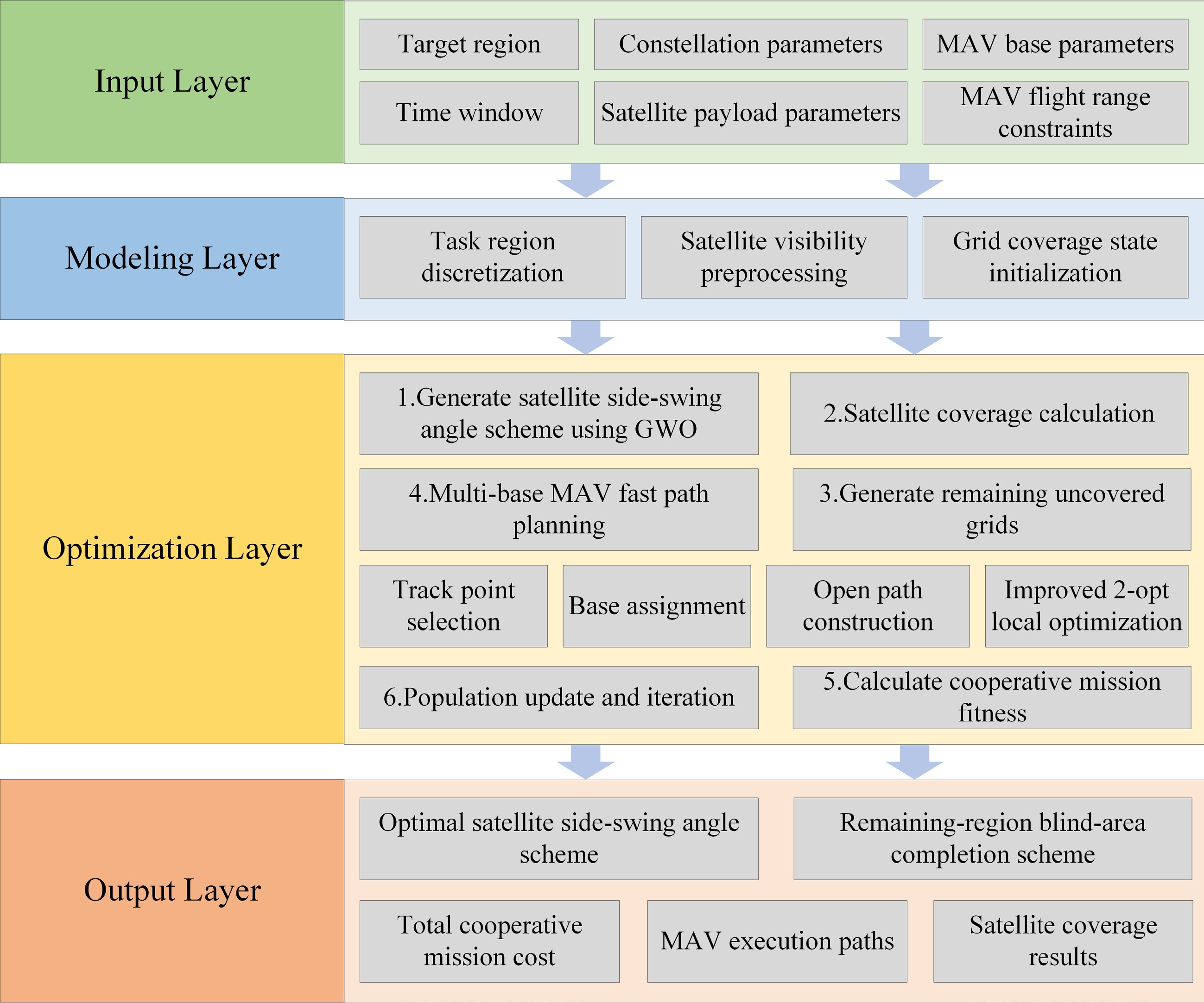
Figure 2. 

Overall framework of the proposed GW-SWCRI method.

With the above operational framework, satellite coverage optimization and MAV path planning form a closed-loop coupling under a unified fitness function, allowing changes in the satellite observation strategy to directly affect the MAV's mission scale and path cost, thereby achieving overall optimization of the satellite-MAV collaborative imaging mission.

Fitness function design

To reflect the overall objective of satellite-MAV collaborative planning, this paper takes the side-swing angle scheme corresponding to each grey wolf individual as the input for pushbroom imaging, obtains the remaining grids after satellite coverage, plans fast supplementary imaging paths for these grids, and takes the total cost of the collaborative mission as the fitness value of each individual. Considering that MAVs' supplementary imaging accounts for the main incremental cost in the collaborative mission, and that a large satellite side-swing angle imposes additional attitude maneuvering burden and potential imaging quality degradation, this paper defines the fitness function as follows:

where $ {D}_{MAV} $ denotes the total flight range of all MAVs, $ At{t}_{i} $ is the side-swing angle of the $ i $^th satellite, $ \sum \left| At{t}_{i}\right| $ denotes the total magnitude of satellite attitude adjustment, $ N $ is the number of satellites, $ {D}_{ref} $ represents the theoretical upper bound of the total MAV range, and $ {\omega }_{1} $ and $ {\omega }_{2} $ are weight coefficients. This fitness function comprehensively reflects the impact of the satellite pushbroom scheme on both the subsequent MAV supplementary imaging efficiency and satellite maneuver cost.

This paper encodes the side-swing angles of the satellite constellation for area observation. The encoding scheme is defined as follows:

where $ wf $ represents an individual grey wolf in the GWO algorithm, $ At{t}_{i} $ denotes the side-swing angle of the $ i $^th satellite, and all $ N $ satellites are visible to the target area during the expected mission period. All side-swing angles are constrained $ Att $ within the range $ [At{t}_{\min },At{t}_{\max }] $.

Position update strategy

Position update method

The core principle of GWO is that all individuals in the population move toward the three leading wolves. The three grey wolves with the best fitness values in the population are denoted as $ \alpha $, $ \beta $, and $ \delta $, respectively, and their corresponding side-swing angles are expressed as $ {b}_{\alpha }(t) $, $ {b}_{\beta }(t) $, and $ {b}_{\delta }(t) $. For the $ i $^th satellite, the distance between each population individual and the three leading wolves is calculated as:

The two key coefficients $ A $ and $ C $ vary with the iteration count and are given by:

where $ ran{d}_{1k}(t) $ and $ ran{d}_{2k}(t) $ are random numbers within the interval [0,1], and $ a(t) $ is the convergence factor, defined as:

where $ {T}_{\max } $ denotes the maximum number of iterations. Using the above parameters, the candidate position of each grey wolf relative to each leading wolf at the $ t $^th iteration are obtained as:

Accordingly, the updated position at the $ (t+1) $^th iteration is given by:

Maximum step-size constrained reflective boundary handling (MSRBH)

To avoid excessively large position jumps in the early iteration stage, which would push updated positions beyond $ [At{t}_{\min },At{t}_{\max }] $ and cause side-swing angles to cluster at the boundaries, a maximum step size constraint is applied to each update step. Let the side-swing angle increment between the $ t $^th iteration and $ (t+1) $^th iterations be defined as:

Let $ {\Delta }_{\max } $ denote the maximum allowable step size. The constrained side-swing angle increment is then given by:

The final side-swing angle after constraint application is then calculated as:

In the traditional GWO, out-of-bounds solutions are typically handled via boundary truncation. Specifically, in the updated positions $ {b}_{i}(t+1) $, any value less than $ At{t}_{\min } $ is clamped to $ At{t}_{\min } $, and any value greater than $ At{t}_{\max } $ is clamped to $ At{t}_{\max } $. When the range $ [At{t}_{\min },At{t}_{\max }] $ is narrow, this mechanism compresses a large number of out-of-bound solutions to the two boundary values, thereby degrading population diversity and convergence performance.

In this paper, a reflection mechanism is proposed to address out-of-bounds solutions. The side-swing angle after reflection-based boundary handling is defined as:

Equation (24) describes a single reflection operation. If the value still exceeds the bounds after one reflection, the process is repeated iteratively until the constraint is satisfied, i.e.,

Compared with direct boundary truncation, this reflective mechanism maps out-of-bounds solutions back into the feasible region based on their out-of-bounds distances, rather than forcing them onto the boundary points; thus, it prevents multiple updated positions from being clustered at $ At{t}_{\min } $ or $ At{t}_{\max } $ and effectively alleviates the boundary adsorption phenomenon.

Overall algorithm flow

The process of the satellite constellation area coverage method using GWO in this paper is as follows:

Step 1: Encode the look angles of the satellite constellation to obtain the initial population;

Step 2: Calculate the coverage fitness of each individual and select the $ \alpha $, $ \beta $, and $ \delta $ wolves;

Step 3: Compute candidate new positions based on the position update formula of GWO;

Step 4: Introduce a maximum step size constraint to limit the single update amplitude;

Step 5: Adopt the reflection boundary handling strategy to map out-of-bounds solutions back to the legal range;

Step 6: Repeat iterative updates until the termination condition is met;

Step 7: Output the optimal combination of look angles and the corresponding coverage result.

In this chapter, within the framework of satellite-MAV collaborative coverage, a rapid path planning method for multi-base MAVs is proposed to address the supplementary imaging requirements for the remaining grids after satellite pushbroom scanning. At each iteration of the GWO algorithm, a satellite coverage strategy is generated, and the resulting spatial distribution of grids requiring supplementary imaging by MAVs serves as the input to the MAV planning module presented in this chapter.

Given the stringent timeliness requirements of satellite constellation observation missions, this chapter designs the MAVs planning module as a fast approximation method that yields high-quality feasible solutions within polynomial time. Under the discrete grid and cross-shaped imaging coverage model, a weighted greedy strategy that integrates coverage benefit and spatial structure information is first adopted to rapidly select imaging waypoints, thereby reducing the total number of waypoints. Subsequently, waypoint assignment and open-path construction are performed under multi-base conditions. Range constraints, turning penalties, and an improved 2-opt strategy are introduced to smooth the paths and reduce operational costs. The module outputs executable trajectories for each MAV along with corresponding cost metrics, which can be directly employed as the MAV supplementary imaging scheme for the collaborative mission. Subject to the constraint that the flight distance does not exceed the maximum range, the algorithm proposed in this chapter minimizes the total flight distance of MAVs, the number of MAV sorties, the total mission completion time, and unnecessary turns in the paths, thereby improving flight smoothness.

Waypoint selection

Optimizing MAV flight trajectories reduces total flight distance. This section exploits the coverage property of individual MAV waypoints over multiple adjacent grids to complete supplementary imaging with the minimum number of waypoints. Meanwhile, a comprehensive evaluation function is designed to optimize trajectories.

When one MAV waypoint is determined, and the next adjacent waypoint needs to be selected, traditional methods rely on exhaustive selection from the set of uncovered grids, leading to a large per-iteration search space and slow convergence. This paper defines candidate waypoints based on coverage characteristics, denoted as:

Using $ {V}_{cand} $ as the candidate set for the next waypoint not only matches the MAV coverage characteristics but also improves search efficiency. For a candidate waypoint $ v\in {V}_{cand} $, its coverage benefit is defined as:

A larger $ {S}_{\mathrm{cov}}(v) $ indicates more newly covered grids after selecting waypoint $ v $, representing a higher benefit. If the algorithm only selects waypoints that cover many new grids, it tends to prioritize large contiguous uncovered areas, leaving the remaining uncovered points distributed along the edges of the target area or scattered as isolated points. This increases unnecessary MAV flights. To address this issue, this paper introduces an edge importance metric in addition to the coverage benefit. For any uncovered grid $ {g}_{x,y}\in {g}_{unc} $, the number of uncovered neighbors in its 4-neighborhood is defined as:

where $ {\mathrm{K }}_{4}(x,y) $ denotes the 4-neighborhood set of grid $ {g}_{x,y} $. The edge importance is then defined as:

That is, a grid with fewer neighbors has higher importance. For a candidate waypoint $ v $, its edge benefit is defined as:

$ {S}_{edge}(v) $ helps prioritize coverage of region boundaries, elongated tails, and isolated targets during candidate waypoint search, which reduces the need for additional boundary processing steps later.

To further improve the algorithm's awareness of spatial structure, this paper builds a connectivity graph for the current uncovered set $ {g}_{unc} $ and uses breadth-first search to identify all connected components. Let $ \Gamma (g) $ denote the connected component to which grid $ g $ belongs; the connectivity region benefit of a candidate waypoint is defined as:

The connectivity region benefit encourages the algorithm to prioritize covering target grids in large-scale connected regions, which helps maintain task continuity and improve the feasibility of subsequent path construction.

When an MAV selects an imaging grid, in addition to the coverage benefit, the spatial distance from the MAV's takeoff base to the imaging grid is also important. A longer distance from the imaging grid to the takeoff base means that more range is required to reach the mission execution location. Therefore, when selecting waypoints, the distance from the grid to its nearest base is defined as:

After distance normalization, the base distance cost for candidate waypoint $ v $, computed from $ {D}_{Base}(g) $, is defined as:

In summary, the comprehensive scoring function for candidate waypoints is constructed as follows:

where $ \alpha $, $ \beta $, $ \gamma $, and $ \mu $ are weight coefficients.

Once the comprehensive scoring function is established, the waypoint with the highest score is selected in each step. This selection process is repeated until $ {g}_{unc}=\varnothing $.

Multi-point open path planning under multiple constraints

Given the set of waypoints, this section addresses the open-path planning problem for MAVs with multiple bases. The objective is to assign all waypoints to different bases and determine the visiting order subject to the maximum range constraint of a single MAV. Let the set of candidate waypoints be denoted as $ {V}^{*} $. For each waypoint $ v\in {V}^{*} $, the nearest base is assigned as its takeoff base, denoted as $ B(v) $, which partitions the global set of waypoints into several subsets:

where $ M $ is the total number of bases. For each base $ {B}_{m} $, let the corresponding set of waypoints be $ {V}_{m} $. An open path is constructed for each MAV sortie, and new waypoints are added sequentially to this path subject to the range constraint. If adding any remaining waypoint would cause the path length to exceed the maximum range, the current path is terminated, and a new sortie is started, until all waypoints in $ {V}_{m} $ have been visited. Let $ u $ denote the last waypoint of the current path, and $ v $ denote a candidate waypoint. Adding $ v $ to the path yields the following incremental distance :

To improve flight path smoothness based on MAV flight characteristics, this paper introduces a turning penalty term in path construction. Let $ {v}_{k-1} $ and $ {v}_{k} $ denote the last two points of the current path, and $ v $ denote the point to be inserted. Under the local planar approximation, the vectors are defined as:

Then the turning angle $ \theta $ is calculated as:

The turning penalty term is defined as:

If the path contains fewer than two waypoints, $ {P}_{turn}(v) $ is set to 0. A straighter path results in lower cost for subsequent waypoints, while waypoints requiring larger turns incur higher penalties. To prevent the path length from approaching the maximum range limit, a range risk penalty mechanism is further introduced. Let the accumulated length of the current path be $ {L}_{cur} $, the range utilization ratio is defined as:

Then the range risk is defined as:

where $ {\rho }_{0} $ denotes the risk trigger threshold. As the MAV approaches its range limit, $ {P}_{risk}(\rho ) $ rapidly increases candidate waypoint costs, which maintains a sufficient safety margin.

Incorporating the three factors of flight distance, turning smoothness, and range risk, the path extension cost for a candidate waypoint $ v $ is defined as:

where $ {\lambda }_{d} $, $ {\lambda }_{t} $, and $ {\lambda }_{r} $ denote the weights of distance, turning penalty, and range risk, respectively. Among all feasible candidate waypoints that satisfy the range constraint, the one with the smallest $ G(v) $ value is selected and added to the current path. If no candidate waypoint satisfies the constraint, the current path is terminated, and a new sortie path is generated.

Improved 2-opt local search method

Following initial path planning, generated paths often contain local detours and unnecessary turns due to their strong dependence on construction order. To further improve path quality, this paper adopts an improved 2-opt local search method to optimize each generated initial path. For path:

two indices $ i $ and $ j $ are selected with $ 1\leq i \lt j\leq n $, and the subsequence of waypoints $ ({v}_{i},{v}_{i+1},\cdots ,{v}_{j}) $ is reversed to generate a new path:

Standard 2-opt uses total flight distance as the sole optimization objective. This work extends it to a joint cost function:

where $ r $ denotes a complete path, $ L(r) $ is the total path length, and $ H(r) $ is the total turning cost of the path, defined as:

In this expression, $ {\theta }_{k} $ denotes the turning angle at waypoint $ {v}_{k} $, and $ {k}_{d} $ and $ {k}_{t} $ are the weight coefficients for path length and turning cost, respectively, which sum to 1. Since local optimization may reduce turning cost at the expense of increased path length, this paper introduces a safety range margin constraint when accepting a new solution. Let the safety margin ratio be $ \eta $, and the constraint is:

where $ L\left({r}^{\prime}\right) $ is the total length of the new path. The 2-opt reversal is accepted only if the new path meets this constraint. The optimization terminates when no further cost-improving reversal can be found, or the maximum number of iterations is reached.

Overview of the MBM-FPP algorithm

The overall workflow of the MBM-FPP algorithm is shown in Fig. 3.

Figure 3. 

Algorithm flow of MBM-FPP.

First, input parameters, including imaging grids, uncovered grid sets, base locations, and MAV range constraints, are loaded. Uncovered areas requiring supplementary observation are extracted based on the constellation coverage results. Next, a set of candidate waypoints is constructed based on the spatial distribution of uncovered grids. The score of each waypoint is calculated by jointly considering its coverage contribution, flight cost, and base accessibility. Key waypoints are selected sequentially until all uncovered grids are fully covered or no valid waypoints can be further selected. Then, the selected waypoints are assigned to corresponding bases based on the distance and travel cost between waypoints and each base. Initial MAV flight paths are constructed for each base. During path construction, the next waypoint with the minimum incremental cost is selected subject to the range constraint. If the current path can no longer be extended, the path is terminated, and a new MAV path is generated, yielding the initial path set for multi-base and multi-MAV scenarios. Finally, the improved 2-opt algorithm is adopted to perform local optimization on the initial paths. All optimized paths are verified against range and cost constraints, and the feasible MAVs path set is output.

The overall time complexity of MBM-FPP is mainly determined by three components: grid coverage determination, task assignment, and MAVs' path planning. Let $ N $ denote the total number of discrete grids, $ M $ denote the number of grids requiring supplementary observation by MAVs, and $ K $ denote the number of MAVs. The time complexity of coverage determination is $ O\left(N\right) $, and the time complexity of task assignment is $ O\left(KM\right) $. When tasks are relatively evenly distributed among MAVs, the time complexity of path planning is approximately $ O({M}^{2}/K) $. Accordingly, the total time complexity of the algorithm can be expressed as $ O(N+KM+{M}^{2}/K) $. Since $ M\leq N $, the overall complexity can be approximated as $ O({N}^{2}) $. This result demonstrates that the algorithm can satisfy the requirement of rapid path planning under reasonable grid discretization.

To sum up, the pseudo code of the Algorithm 1 proposed in this paper is as follows:

This paper designs two scenarios to verify the correctness of the proposed framework and algorithm, as well as their generalizability to different satellite swath widths, side-swing angles, and base distributions. Multiple simulations are conducted for each scenario to validate the effectiveness and stability of the algorithm. Comparisons with the genetic algorithm and the greedy search algorithm are also performed. The simulation results show that the proposed algorithm achieves better convergence performance.

To verify the correctness, effectiveness, and scenario adaptability of the proposed satellite-MAV collaborative search mission planning framework and optimization algorithm, this paper designs two typical simulation scenarios for experimental analysis. The two scenarios differ in satellite swath width, side-swing angle constraints, and the spatial distribution of MAV takeoff bases, and are used to test the generalizability of the proposed method under different mission conditions. Meanwhile, to reduce the impact of randomness in individual simulations, multiple independent repeated simulations are conducted for each scenario, and the simulation results are averaged to further validate the stability and reliability of the algorithm. In addition, to evaluate the optimization performance of the proposed algorithm, comparisons are made with two typical benchmark methods: the genetic algorithm and the greedy search algorithm.

Algorithm validation

The two simulation scenarios use the same simulation time window, heterogeneous constellation configuration, and observation target. The simulation period is set from 2026-03-27 00:00:00 to 2026-03-28 00:00:00 (UTC). Scenario time is counted from 0 s at the simulation start, with a time step of 1 s. The target observation area is a spherical quadrilateral region, with longitude ranging from 170.5 deg to 175.5 deg and latitude ranging from −2.5 deg to 2.5 deg. The mission satellites form a heterogeneous constellation consisting of two Walker constellations, denoted Walker1 and Walker2. The initial satellite parameters and constellation settings for Walker1 and Walker2 are listed in Table 1. The satellite visibility ranges and corresponding imaging swath widths for Scenarios 1 and 2 are given in Table 2.

Each MAV has a maximum flight range of 600 km and an average flight speed of 25 m/s. The maximum range already includes reserved return-flight energy, so no additional return segment is added during path planning. MAVs take off from their respective bases, with no limit on the number of sorties per base. The base configurations for the two scenarios are listed in Table 3.

The initialization parameters of the MBM-FPP method are summarized in Table 4.

The algorithm is set to terminate after 200 iterations, with a population size of 20. The simulation results for the two scenarios are presented in Fig. 4. As shown in the figure, the fitness curves for both scenarios drop rapidly in the early stage and gradually level off later, indicating that the proposed algorithm has fast initial search capability and can converge steadily to a stable solution in subsequent iterations. Specifically, the fitness value in Scenario 1 decreases from 0.837 to 0.742, a reduction of approximately 11.35%; in Scenario 2, it decreases from 0.694 to 0.594, a reduction of approximately 14.41%. This confirms that the proposed algorithm has strong optimization performance across different scenarios. Meanwhile, the initial fitness values and final convergence results differ between the two scenarios. This is mainly caused by the different distributions of MAV takeoff bases, which result in different effective search ranges for each base. These differences further shape the solution space distribution and overall fitness level of the mission planning problem. Accordingly, the convergence starting points and final convergence results of the algorithm are not fully consistent across different scenarios.

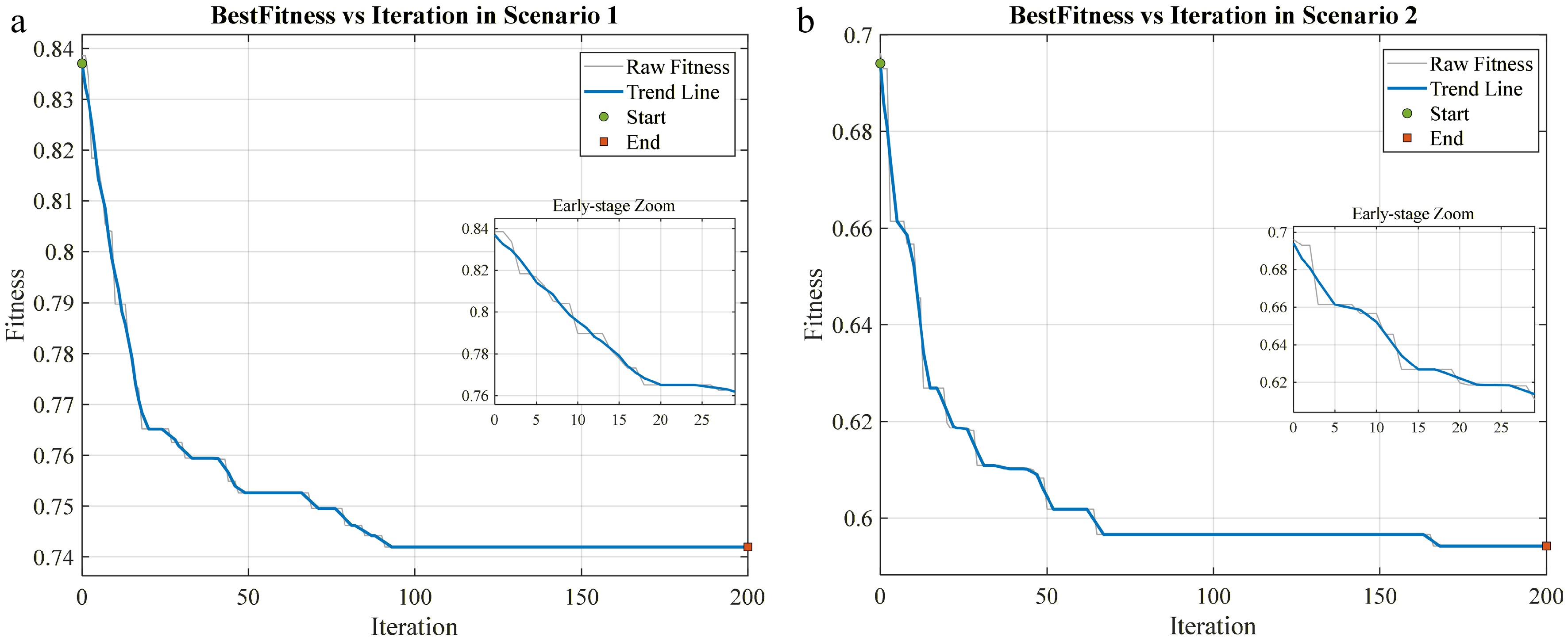
Figure 4. 

Fitness value variation with iterations.

The spatial division results of satellite-MAV collaborative search under the two scenarios are shown in Fig. 5. As shown in the figure, the proposed method can reasonably partition the overall mission area based on satellite coverage capability, MAV takeoff base locations, and mission area distribution. The boundaries of the search ranges corresponding to different MAV bases are relatively clear, forming a clear spatial division of labor across search areas, indicating that the proposed framework can effectively achieve collaborative allocation of satellite search capability and MAVs' maneuverable search capability. Further analysis reveals that due to differences in satellite swath width, side-swing angle, and base distribution between the two scenarios, the final search coverage results also exhibit certain differences. When the base locations, search area shape, or satellite coverage constraints change, the search ranges assigned to each base adjust accordingly, resulting in different spatial coverage structures in the two scenarios. This indicates that the proposed algorithm is not only applicable to a single fixed scenario but can also adaptively adjust the search area allocation scheme according to changes in mission conditions, verifying good generalizability and engineering applicability.

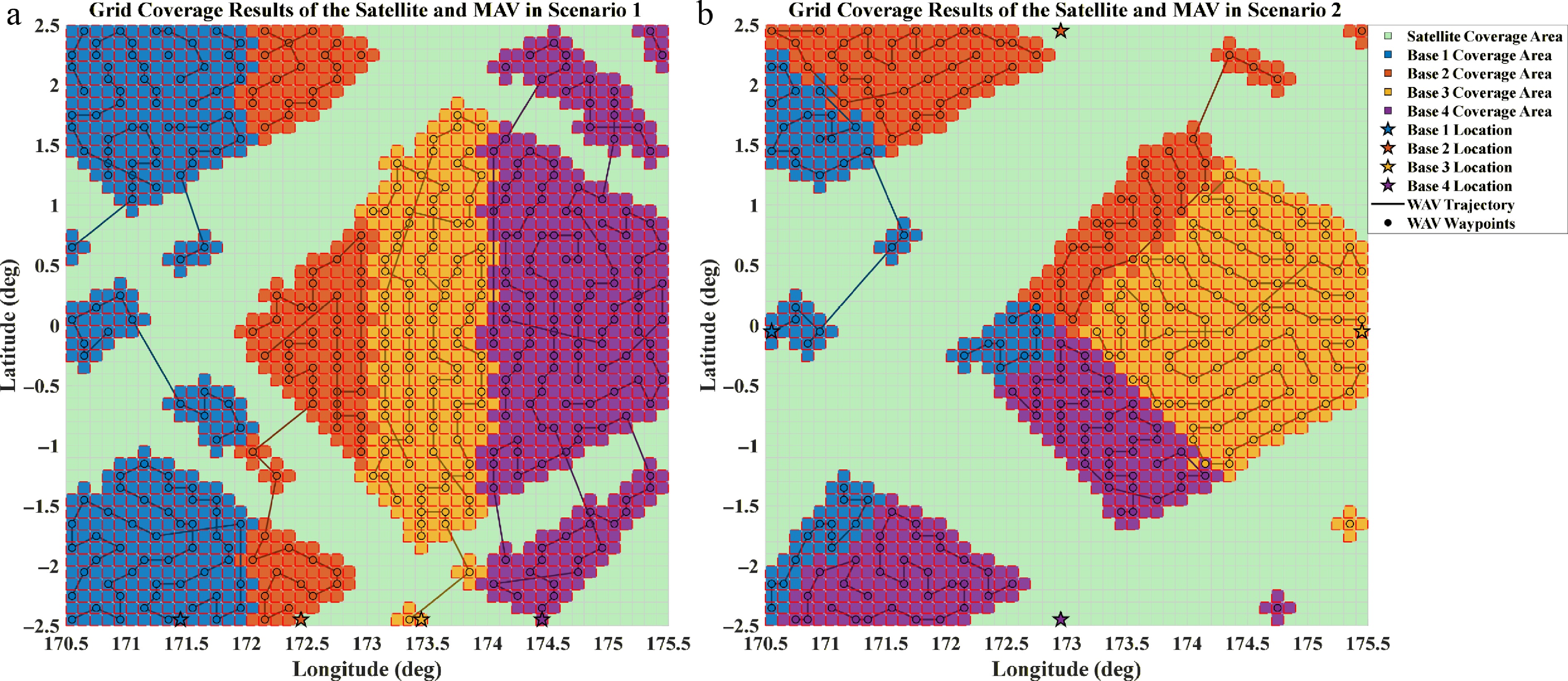
Figure 5. 

Satellite and MAV grid coverage results.

To reduce the impact of random initialization and stochastic search processes on simulation results, this paper performs 10 independent repeated simulations for each scenario and averages the fitness values across all runs. The curves of average fitness vs iterations for the two scenarios are shown in Fig. 6. As shown in the figure, after averaging over multiple repeated simulations, the average fitness curves in both scenarios still decline rapidly in the early iterations and gradually level off in later iterations, indicating that the proposed algorithm maintains a consistent search direction and convergence trend under different random initial conditions, demonstrating good convergence stability. Specifically, the average fitness in Scenario 1 decreases from 0.826 to 0.745, a reduction of 9.81%; in Scenario 2, it decreases from 0.6857 to 0.5934, a reduction of 9.23%. This indicates that the proposed algorithm achieves effective optimization under different mission scenarios. Furthermore, analysis of standard deviation shows that, as the number of iterations increases, fitness fluctuations gradually diminish, and dispersion across repeated simulation runs continues to decrease, indicating that the algorithm can stably converge to a near-optimal solution in later iterations and is less affected by random factors. Therefore, the reliability and robustness of the proposed algorithm are further validated.

Figure 6. 

Variation of fitness value with iterations.

Figures 7 and 8 show the iterative variations in the optimal MAVs cost term and the average optimal MAV range, respectively. As shown in the figures, as iterations progress, the MAVs cost term decreases overall and gradually converges, indicating that the algorithm can effectively reduce the relative range cost for MAVs mission execution. Although the average optimal MAV range exhibits some fluctuations during iteration, it gradually stabilizes in later stages, indicating that the task allocation and path planning results eventually reach a steady state. These results demonstrate that the proposed algorithm performs well in both MAV range cost optimization and path planning stability.

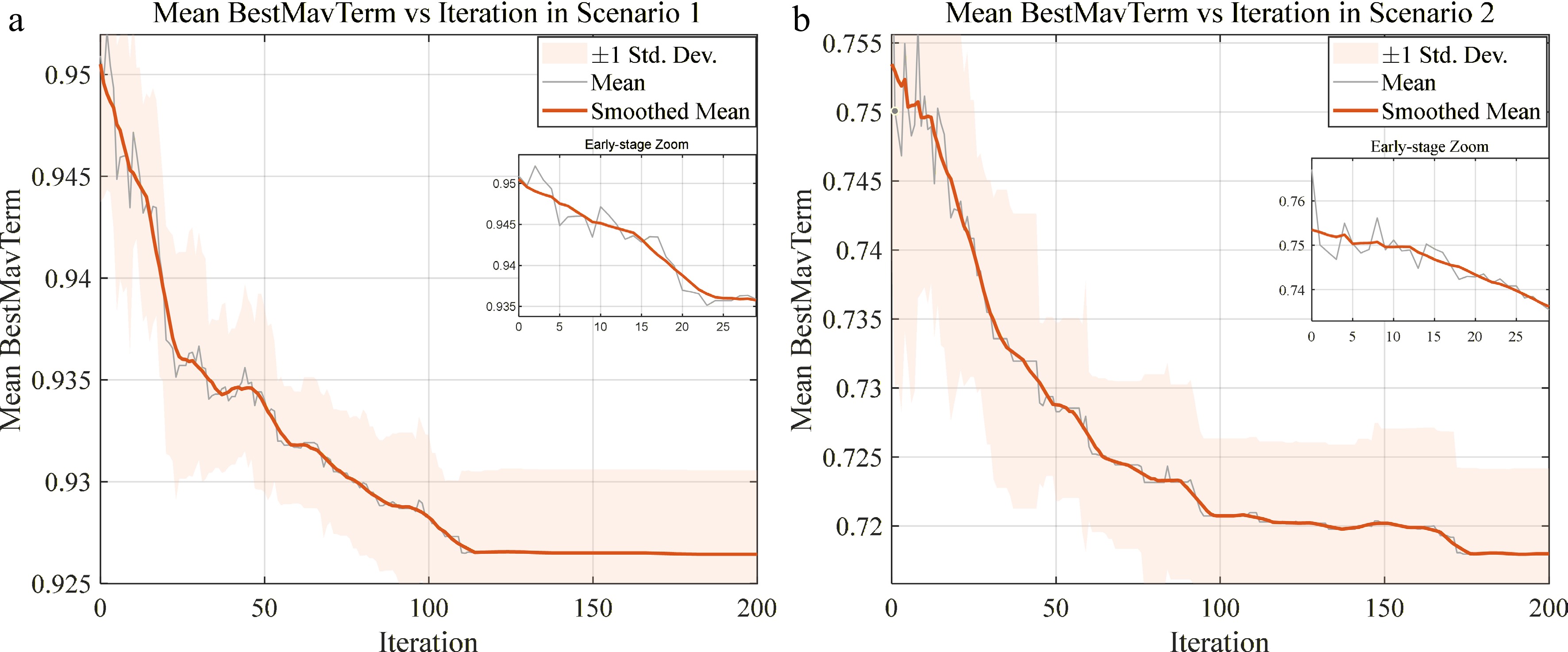
Figure 7. 

Average optimal MAV cost term vs iteration number.

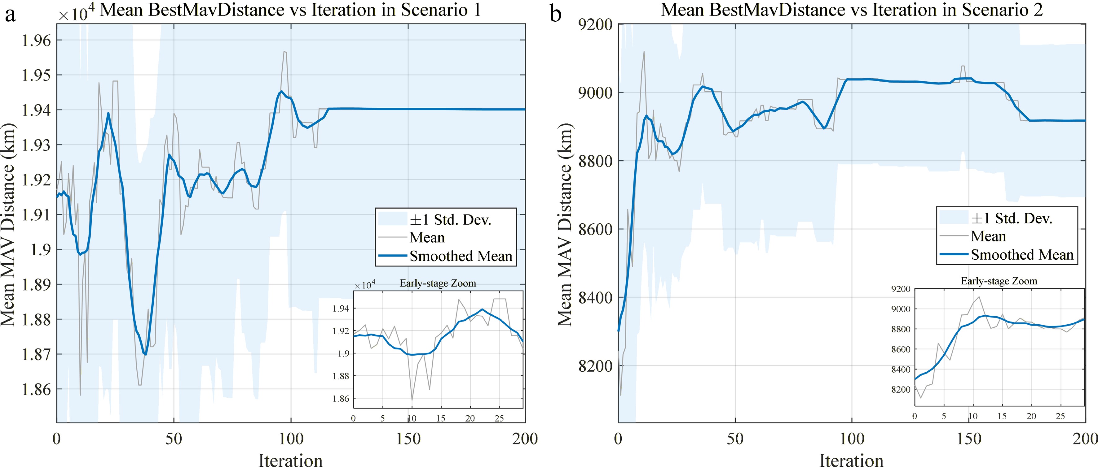
Figure 8. 

Curve of average optimal MAV distance vs iteration number.

The variation in fitness of the three leading wolves $ \alpha $, $ \beta $, and $ \delta $ in the population across iterations is shown in Fig. 9. The results in both scenarios indicate that the fitness values of these three elite individuals continuously decrease as iterations progress and gradually stabilize in the later stage. As the number of iterations increases, the gaps among the three curves gradually narrow, indicating that differences in solution quality among elite individuals are shrinking, and the population gradually transitions from the global exploration phase to the local exploitation phase. Eventually, the fitness curves of the three types of individuals all tend to stabilize, indicating that the algorithm has formed a relatively stable search direction and achieved convergence. The curves of $ \alpha $, $ \beta $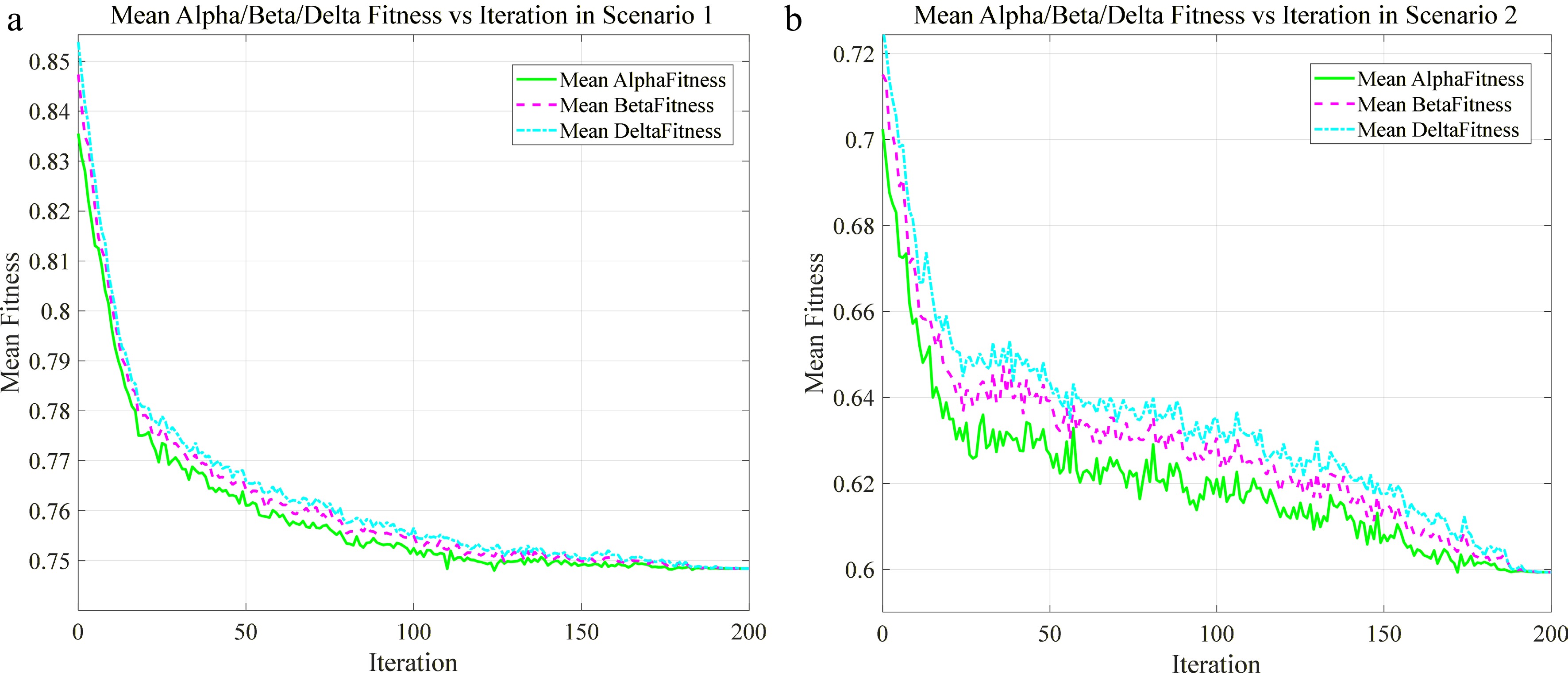, and $ \delta $ in both scenarios exhibit consistent convergence patterns, confirming that the proposed algorithm has good population evolution capability and scenario adaptability under different mission conditions.

Figure 9. 

Variation of fitness of the three leader wolves with iterations.

Comparative simulations are performed to evaluate the convergence performance and runtime of GWO against GS and GA. The proposed GWO uses a population size of 20. GA is tested with two population sizes, 20 and 50. As a deterministic heuristic method, GS does not involve a population parameter.

The results show that the GA with a population size of 20 does not fully converge after 200 iterations, indicating limited optimization efficiency under a small population. The fitness curve of GS declines rapidly in the early iteration stage but converges relatively early, with a high final fitness value, which means that it is prone to falling into local optima. In contrast, the proposed algorithm with the same population size of 20 converges rapidly and achieves the lowest final fitness value, demonstrating better convergence capability and optimization performance.

The computation time results of different algorithms are listed in Table 5. Combined with the results in Fig. 10, although GS has the shortest computation time, its global optimization ability is the weakest and its final convergence accuracy is the poorest; when the population size is set to 20 for both GWO and GA, the total computation time of GWO is slightly longer than that of GA and GS, but the time difference remains within an acceptable range. In terms of optimization performance, the final convergence accuracy of GWO is significantly better than that of GA and GS with the same population size, with a faster convergence rate and stronger deep search capability. Even when the population size of GA is increased to 50 to enhance its search ability, its final optimization performance is still inferior to that of GWO with a population size of only 20. Overall, the proposed algorithm can complete effective optimization with a smaller population size and is more suitable for fast planning demands in time-sensitive tasks such as satellite observation.

Figure 10. 

Fitness variation curves with iterations for different algorithms.

Discussion

Based on the comprehensive simulation results presented above, the proposed collaborative search planning framework and optimization algorithm demonstrate good effectiveness, stability, and generalizability across the two different scenarios. First, in terms of fitness variation in both single-run and multiple repeated simulations, the algorithm exhibits rapid initial optimization in the early stage and stable convergence in the later stage, indicating strong global exploration and local exploitation capability. Second, in terms of the collaborative search area partitioning results, the algorithm can adaptively divide the mission area according to satellite observation capabilities, side-swing angle constraints, and the distribution of MAV bases, thereby achieving a rational allocation of search resources between the satellite and MAVs. Comparative results with the genetic algorithm and greedy search algorithm further show that the proposed algorithm can achieve lower fitness values with smaller population sizes and fewer iterations, while maintaining stable convergence in later iterations, demonstrating better convergence speed and final optimization capability. Therefore, the method proposed in this paper can be effectively applied to collaborative search mission planning problems under different satellite parameters, different side-swing angle constraints, and different base distribution conditions, demonstrating promising potential for engineering applications.

This paper investigates the collaborative search mission planning problem for agile satellites and MAVs, establishes a satellite-MAV collaborative planning model, and proposes corresponding optimization methods. By integrating satellite area coverage and MAV supplementary imaging into a unified framework, this work realizes a collaborative planning scheme in which satellites perform initial coverage and MAVs conduct supplementary imaging. Simulation results demonstrate that the proposed method exhibits good effectiveness, stability, and adaptability under different mission scenarios, achieving rapid convergence with a relatively small population size and yielding superior collaborative planning results. Compared with the genetic algorithm and the greedy search algorithm, the proposed method shows advantages in convergence speed and optimization performance, and can effectively meet the rapid planning requirements of regional collaborative search missions. In summary, this study provides a feasible approach for collaborative search mission planning of agile satellites and MAVs, and also lays a foundation for subsequent research on collaborative mission optimization in complex dynamic scenarios.