Elastic multi-source fusion navigation system based on factor graph optimization

Robotic mobile platforms, including ground vehicles and micro air vehicles (MAVs), increasingly require continuous and accurate pose estimation in long-term autonomous operation. Compared with ground platforms, MAVs impose stricter requirements on navigation robustness because their limited payload, high-maneuverability, and rapid viewpoint changes make them more sensitive to sensor degradation^[1]. However, practical operation environments are often uncertain^[2], such as the Global Navigation Satellite System (GNSS) signal blockage, the loss of visual features caused by dramatic changes in illumination, and the degradation of Light Detection and Ranging (LiDAR) geometric features caused by open areas. Single-sensor navigation or fixed sensor integrated navigation schemes are prone to collapse in these environments. Therefore, a multi-source fusion framework should not only combine complementary observations but also adjust different sensor factors according to their real-time consistency.

In the field of two-sensor integrated navigation, Visual-Inertial Odometry (VIO) and LiDAR-Inertial Odometry (LIO) have made significant progress. VINS-Mono^[3] formulates monocular visual-inertial state estimation as a sliding-window nonlinear optimization problem, while ORB-SLAM3^[4] improves visual and visual-inertial simultaneous localization and mapping (SLAM) through multi-map management. However, visual-inertial methods are still sensitive to weak texture, illumination variation, and insufficient parallax. In terms of LIO, LIO-SAM^[5] introduces a factor graph framework to integrate LiDAR and inertial measurements, and FAST-LIO2^[6] improves mapping efficiency by using the ikd-tree^[7]. Nevertheless, LiDAR-inertial methods still depend on sufficient geometric structure and lack absolute position constraints, which may lead to accumulated drift in open, repetitive, or geometrically degenerate environments.

To improve robustness, heterogeneous multi-sensor fusion has attracted increasing attention. LIC-Fusion^[8] proposed a LiDAR-visual-inertial coupled framework based on the Multi-State Constraint Kalman Filter (MSCKF), and R3LIVE^[9] further improves local odometry robustness by combining LiDAR geometric mapping with visual texture information. However, these visual-LiDAR-inertial systems mainly focus on local relative motion estimation, and global positioning observations are not explicitly managed in the same optimization framework. GVINS^[10] couples GNSS raw measurements with VIO information to improve global consistency, but LiDAR geometric constraints are not included. More recent studies further extend multi-sensor fusion toward different sensor combinations. LE-VINS^[11] introduces solid-state LiDAR information to enhance visual-inertial navigation, while GLIO^[12] tightly integrates GNSS, LiDAR, and Inertial Measurement Unit (IMU) measurements for continuous state estimation in urban environments. LIGO^[13] further investigates LiDAR-inertial-GNSS odometry with a hierarchical fusion structure for global localization and real-time mapping. These studies show that heterogeneous fusion can improve navigation robustness, but most existing systems are still designed for specific sensor combinations rather than a unified framework that can jointly manage visual, LiDAR, GNSS, and inertial factors.

Another limitation lies in calibration and degradation handling. Offline calibration methods such as Kalibr^[14] can provide accurate initial spatio-temporal parameters, but they are difficult to adapt to possible parameter offsets caused by mechanical vibration, timestamp inconsistency, or installation changes during long-term operation. Recent tightly coupled systems and optimization frameworks^[13,15−17] have improved estimation accuracy and extensibility. However, their factor topology is usually predefined by the sensor configuration, and the response to GNSS outliers, visual feature loss, or LiDAR geometric degeneracy is still limited. Keeping all unreliable factors may introduce inconsistent constraints, whereas directly disabling a sensor stream may discard useful partial observations. Therefore, a key unresolved problem is how to maintain accurate and continuous pose estimation when heterogeneous sensor factors become partially unreliable or when spatio-temporal inconsistency occurs.

In response to the above challenges, this paper proposes an elastic multi-source fusion navigation framework based on Factor Graph Optimization (FGO). The framework incorporates visual, LiDAR, GNSS, and inertial factors into a common sliding-window optimization, while estimating the spatio-temporal parameters between heterogeneous sensors online. The main contributions are summarized as follows:

A unified sliding-window factor graph is constructed by incorporating visual, LiDAR, GNSS, and inertial factors for joint trajectory estimation.

Camera-IMU and LiDAR-IMU extrinsic parameters and temporal offsets are included in the state vector to support online spatio-temporal calibration.

A residual-consistency-based elastic factor management strategy is introduced to suppress inconsistent measurement factors and support active topology adjustment under partial sensor degradation.

Experiments on public ground mobile platform and MAV datasets evaluate trajectory accuracy, online calibration behavior, topology-switching robustness, and runtime performance.

The system adopts factor-graph-based tightly coupled optimization as the core architecture, where IMU, camera, LiDAR, and GNSS measurements are modeled as different factors, as shown in Fig. 1.

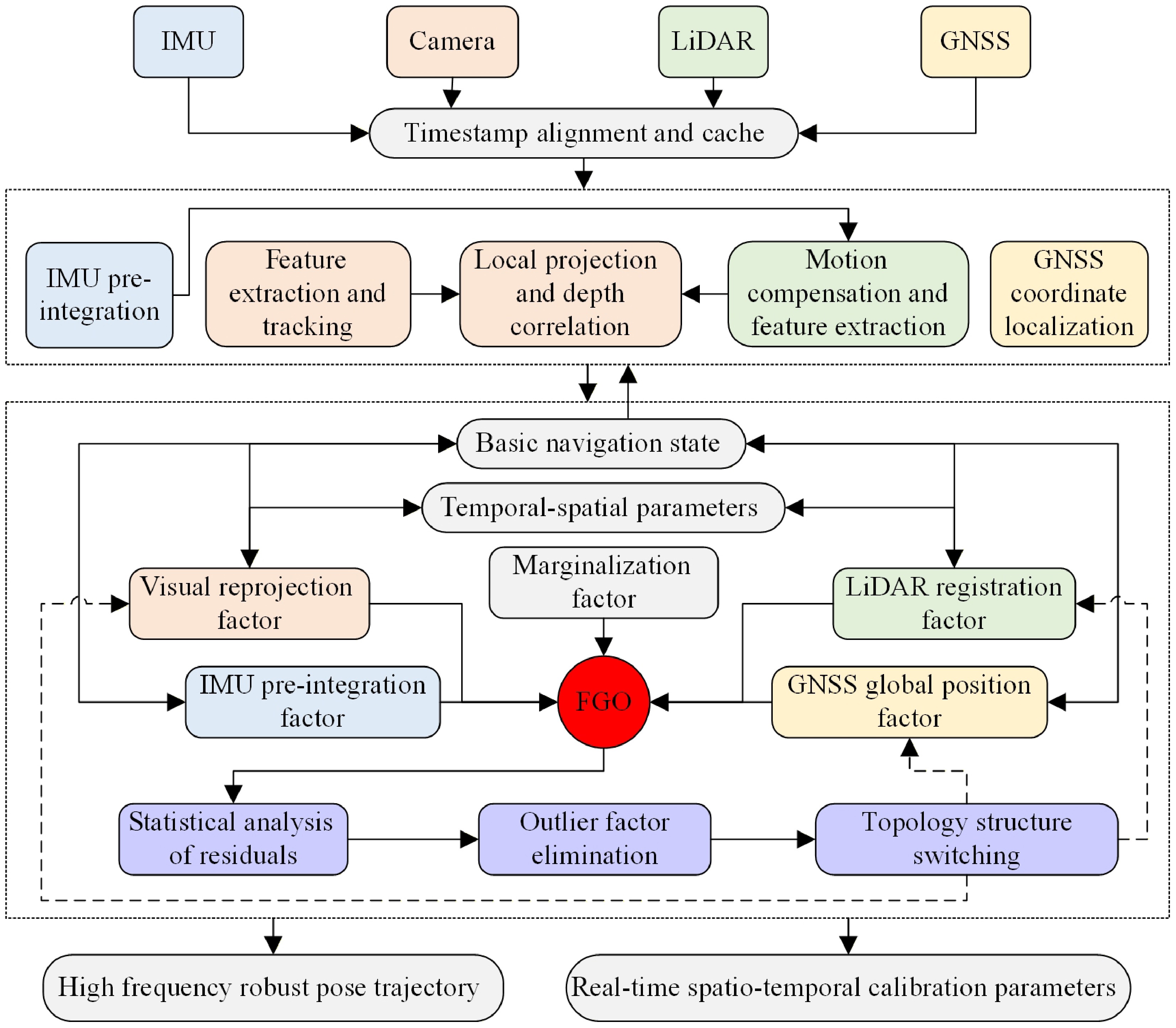
Figure 1. 

Overview of elastic multi-source fusion navigation system.

In the front-end preprocessing stage, the pose prior from IMU pre-integration is used to compensate for LiDAR scan distortion and extract geometric features. The local point cloud is projected onto the image plane to provide depth cues for visual feature tracking. In addition, the system defines the extrinsic parameters and time offset between sensors as the state variables to be optimized, and constructs the residual model together with the motion state in the sliding window. This design allows the spatio-temporal parameters to be refined during operation through multi-modal observation constraints. The back-end uses sliding-window optimization to jointly estimate the full state vector from the active measurement factors. To cope with sensor degradation, an elastic variable-structure management module evaluates residual consistency and updates the active factor topology. When GNSS, visual, or LiDAR constraints become unavailable or inconsistent, the corresponding unreliable factors are removed from or disabled in the active graph. The system continuously outputs pose estimates and online spatio-temporal calibration parameters through the sliding-window update.

In order to describe the kinematics model of the multi-sensor in a unified space, the following coordinate system is defined: the origin of the world coordinate system {w} is located at the starting point of the system, the X-axis and the Y-axis point to the local geographical east and north, respectively, and the Z-axis is aligned with the gravity vector. The body coordinate system {b} is strictly bound to the IMU center, and follows the standard agreement of front-right-down inertial navigation as the main reference frame for system state estimation. The camera coordinate system {c} and the LiDAR coordinate system {l} are the local physical coordinate systems of the visual sensor and the LiDAR, respectively, and are associated with the body coordinate system through the extrinsic parameters. In the following equations, the superscript denotes the coordinate frame in which a vector is expressed, while the subscript identifies the physical frame, sensor, or time index.

In the sliding-window optimization process, the complete state vector of the system is composed of the basic navigation state, the spatio-temporal parameters between sensors, and the depth of visual features. It defines the basic navigation state of the i frame moment as:

where, $ \boldsymbol{p}_{b_i}^w $, $ \boldsymbol{v}_{b_i}^w $ and $ \boldsymbol{q}_{b_i}^w $ represent the position, velocity, and rotation quaternion of the body system relative to the world system. $ \boldsymbol{b}_{a_i} $ and $ \boldsymbol{b}_{g_i} $ represent the bias of the accelerometer and gyroscope.

The spatio-temporal state of the camera and the LiDAR is parameterized online. Considering the dynamic delay of the shutter trigger and data transmission in the carrier motion, two independent time offset parameters are introduced between the camera and the IMU to capture the delay fluctuation between adjacent observation frames. The spatio-temporal state quantity on the camera side is defined as:

where, $ \boldsymbol{q}_c^b $ and $ \boldsymbol{p}_c^b $ denote the rotation and translation from the camera frame to the body frame. $ \delta {t}_{{{c}_{i}}} $ and $ \delta {t}_{{{c}_{j}}} $ denote the temporal offset between the camera timestamp and the IMU time reference at different times. A set of standard extrinsic parameters and a single time offset parameter between LiDAR and IMU are defined as:

where, $ \boldsymbol{q}_l^b $ and $ \boldsymbol{p}_l^b $ denote the rotation and translation from the LiDAR frame to the body frame. $ \delta {t}_{l} $ denotes the temporal offset between the LiDAR timestamp and the IMU time reference. The motion states, IMU biases, extrinsic parameters, and temporal offsets are optimized online, while sensor intrinsic parameters, gravity, and initial noise statistics are treated as known parameters or priors.

IMU plays a key role in motion modeling and state transfer in the whole fusion system. It outputs the raw angular velocity and linear acceleration with high-frequency, considering the measurement noise and bias. The IMU mechanical arrangement equation is used to realize the high-frequency continuous output of the system. For time t in the interval [i, j], according to the integral relation, the iterative formulas of position, velocity, and attitude are obtained:

where, $ \otimes $ represents quaternion multiplication. $ \boldsymbol{R}_{b_t}^w $ denotes the rotation matrix corresponding to the attitude quaternion $ \boldsymbol{q}_{b_t}^w $, $ \hat{\boldsymbol{\omega}}_t $ and $ \hat{\boldsymbol{a}}_t $ are the measured angular velocity and specific force from the IMU. $ \boldsymbol{b}_{g_t} $ and $ \boldsymbol{b}_{a_t} $ are the time-varying gyroscope and accelerometer bias, $ \boldsymbol{\eta}_g $ and $ \boldsymbol{\eta}_a $ represent Gaussian white noise, and $ \boldsymbol{g}^w $ is the gravity vector in the world coordinate system.

Multi-source heterogeneous residual construction

This section presents the residual construction of the IMU, visual, LiDAR, and GNSS factors. To support online calibration, the spatial transformations and temporal offsets of the camera and LiDAR are explicitly embedded into the corresponding residual models.

IMU pre-integration

To avoid repeated integration during optimization, the IMU measurements between two keyframes are pre-integrated as relative motion increments^[3]. Since the bias is updated during optimization, first-order correction is used to update the pre-integrated terms, and the IMU residual is constructed as:

The IMU residual describes the deviation between the predicted state transition and the pre-integrated measurement. This factor provides short-term motion propagation when visual or LiDAR constraints become weak.

Visual reprojection feature constraint

A monocular camera lacks direct scale information and may suffer from scale drift under challenging motion^[18]. To improve feature depth estimation, the local LiDAR point cloud is used to provide depth cues for the visual feature point $ \boldsymbol{f}^{c_i} $ extracted in frame i. According to the extrinsic parameters of the camera $ \{\boldsymbol{p}_{c}^{b},\;\boldsymbol{q}_{c}^{b}\} $, the feature point is projected into the body coordinate system. Neighboring LiDAR points around the projection ray are searched, and a local tangent plane is fitted. The inverse depth $ {\lambda }_{i} $ of the visual feature is then obtained from the intersection between the projection ray and the fitted plane. If reliable LiDAR depth is unavailable, feature depth is estimated by visual triangulation.

The process of visual reprojection is to project the three-dimensional feature points in space from one moment to the camera imaging plane at another moment, and calculate the deviation between the predicted position and the actual observation position^[19]. The pixel coordinate of the m feature point $ \boldsymbol{p}_m^{c_i} $ observed in the image of frame i is $ [u_m^{c_i},\;v_m^{c_i}]^{\mathit{\mathrm{T}}} $, and its normalized coordinate is $ [cx_m^{c_i},\;y_m^{c_i},1]_{ }^{\mathrm{T}} $. The three-dimensional space point coordinate $ \boldsymbol{f}_m^{b_i} $ of the point in the body coordinate system at time i can be restored by using the inverse depth corresponding to the feature point and the extrinsic parameters of the camera. Further, the position in the world coordinate system is obtained by the pose in the navigation state $ \{\boldsymbol{p}_{{b}_{i}}^{w},\;\boldsymbol{q}_{{b}_{i}}^{w}\} $ at time i. When the carrier moves to frame j, the coordinate in the body coordinate system at time j can be obtained by using the navigation state pose $ \{\boldsymbol{p}_{{b}_{j}}^{w},\;\boldsymbol{q}_{{b}_{j}}^{w}\} $, and then the feature point reprojection coordinate is obtained by projecting to the j-frame camera plane:

In the ideal case of strict time alignment, visual reprojection residuals can be established as:

where, $ \hat{\boldsymbol{p}}_m^{c_j} $ is the obs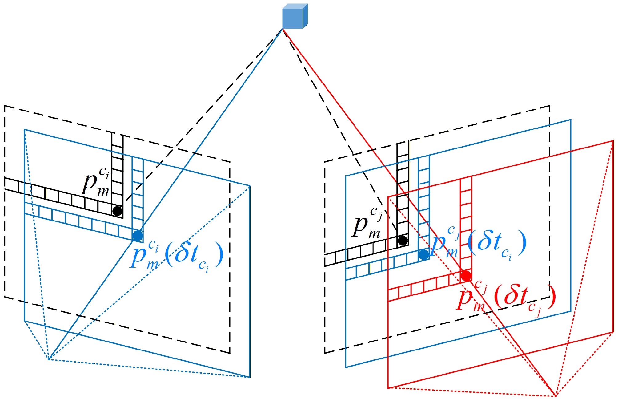erved value of the feature point, and $ proj(\cdot ) $ is the projection function containing the internal parameter of the camera, which converts the normalized coordinates into pixel coordinates. In practice, the image timestamp may be offset from the IMU time reference^[20]. During platform motion, this offset introduces biased reprojection residuals, so pixel-level delay compensation is applied, as shown in Fig. 2.

Figure 2. 

Visual reprojection process considering time delay.

The camera usually shares a time offset for the whole frame of the synchronous exposure whole image, but considering that there may be an uneven time offset between different frame images, the actual observed pixel coordinates $ \boldsymbol{p}_m^{c_k} $ are captured at the moment $ {t}_{k}+\delta {t}_{{{c}_{k}}} $, and the pixel coordinates are first-order corrected by the pixel velocity. The observed pixel coordinates are then aligned with the state time $ {t}_{k} $ by compensating for the pixel displacement induced by platform motion during the delay interval. Assuming that the time offsets of the i frame and the j frame are $ \delta {t}_{{{c}_{i}}} $ and $ \delta {t}_{{{c}_{j}}} $, respectively, then the feature points after delay compensation at moments i and j are obtained:

Therefore, in the visual reprojection residual, the time delay parameter of the camera is also optimized as a variable to be optimized. By minimizing the compensated reprojection residuals, the camera extrinsic parameters and temporal offset can be refined together with the navigation states.

LiDAR geometric feature constraint

LiDAR acquires points sequentially. During platform motion, points within one scan are captured at different times, causing motion distortion that needs to be compensated^[21]. The starting time of point cloud acquisition in a frame is $ {t}_{k} $, the sampling offset of the n point $ \boldsymbol{f}_n^{l_{k,n}} $ in the frame relative to the starting time is $ \Delta {t}_{n} $, and considering the LiDAR time delay$ \delta {t}_{l} $, the actual physical sampling time is:

In order to eliminate the motion distortion, $ \boldsymbol{f}_n^{l_{k,n}} $ is compensated to the local LiDAR coordinate system at the starting time $ {t}_{k} $ of the frame. The state prediction interpolation of IMU pre-integration is used to calculate the state at the sampling time. The compensated point coordinate is:

where, $ \boldsymbol{T}_l^b $ is the LiDAR extrinsic parameter, $ \boldsymbol{T}_{b_{k,n}}^w $ is the instantaneous pose at time $ {t}_{k,n} $ obtained by linear extrapolation of the state quantity at time $ {t}_{k} $. After completing the distortion compensation, the system characterizes the point cloud as a plane point. In order to make full use of the LiDAR point cloud information to construct the residual constraint and select the frame-to-frame matching mode, the LiDAR residual is defined as the orthogonal distance of the feature point $ \boldsymbol{f}_n^{l_i} $ after the motion distortion compensation of the i frame is converted to the feature point $ \boldsymbol{f}_n^{l_j} $ in the j frame, which corresponds to the target plane. The frame-to-frame matching conversion of LiDAR is similar to the process of visual reprojection:

For the feature point $ \boldsymbol{f}_n^{l_j} $ after LiDAR matching transformation, the corresponding correlation plane is found, which is defined by its normal vector $ \boldsymbol{n}_{l_j}^{ } $ and the center point $ \boldsymbol{q}_{l_j}^{ } $ on the plane. Then the LiDAR residual is defined as:

The influence of the fixed time delay between the LiDAR and the IMU on the coordinate transformation is also considered. As shown in Fig. 3, the rotation matrix and the translation vector of the body are compensated:

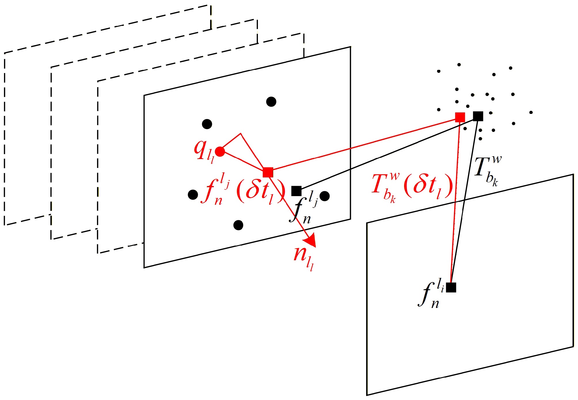
Figure 3. 

LiDAR point cloud matching transformation considering time delay.

In the LiDAR residual, the LiDAR-IMU extrinsic parameters and temporal offset are embedded in the transformation model, allowing them to be refined during sliding-window optimization. Different from the visual feature position compensation model, the LiDAR residual is corrected at the pose level, and the position and attitude are corrected by velocity and angular velocity to conform to the motion process.

GNSS global observation constraint

Visual and LiDAR odometry provide local relative constraints, which may accumulate drift during long-distance operation^[12]. GNSS provides global position observations that can help constrain long-term trajectory drift. In the initialization process of the system, the longitude and latitude height observations are converted to the world coordinate system of the system, and the GNSS position observations are used as the position constraint access factor graph optimization.

GNSS antenna installation usually has a certain spatial offset from the body coordinate system, and the lever-arm effect is considered in the construction of the observation model. The offset vector of the antenna relative to the body coordinate system is defined as $ \boldsymbol{l}_{GNSS}^b $. At time $ {t}_{k} $, the predicted position of the GNSS antenna center in the world coordinate system is obtained by superimposing the rotating lever-arm vector with the current position of the body. The residual is constructed by combining the actual observation value $ \hat{\boldsymbol{p}}_{GNSS}^w $ of GNSS in the world coordinate system^[22]. The GNSS residual is defined as the difference between the predicted antenna position and the GNSS observation:

The GNSS factor provides an absolute position constraint on the body state, and the lever-arm term also introduces attitude-related coupling.

Full coupling factor graph optimization

The system formulates heterogeneous sensor measurements as factors in a nonlinear optimization problem and estimates the navigation state through the factor graph model shown in Fig. 4. The core is to construct a joint cost function in which residuals from different sensor modalities are optimized over a shared state vector.

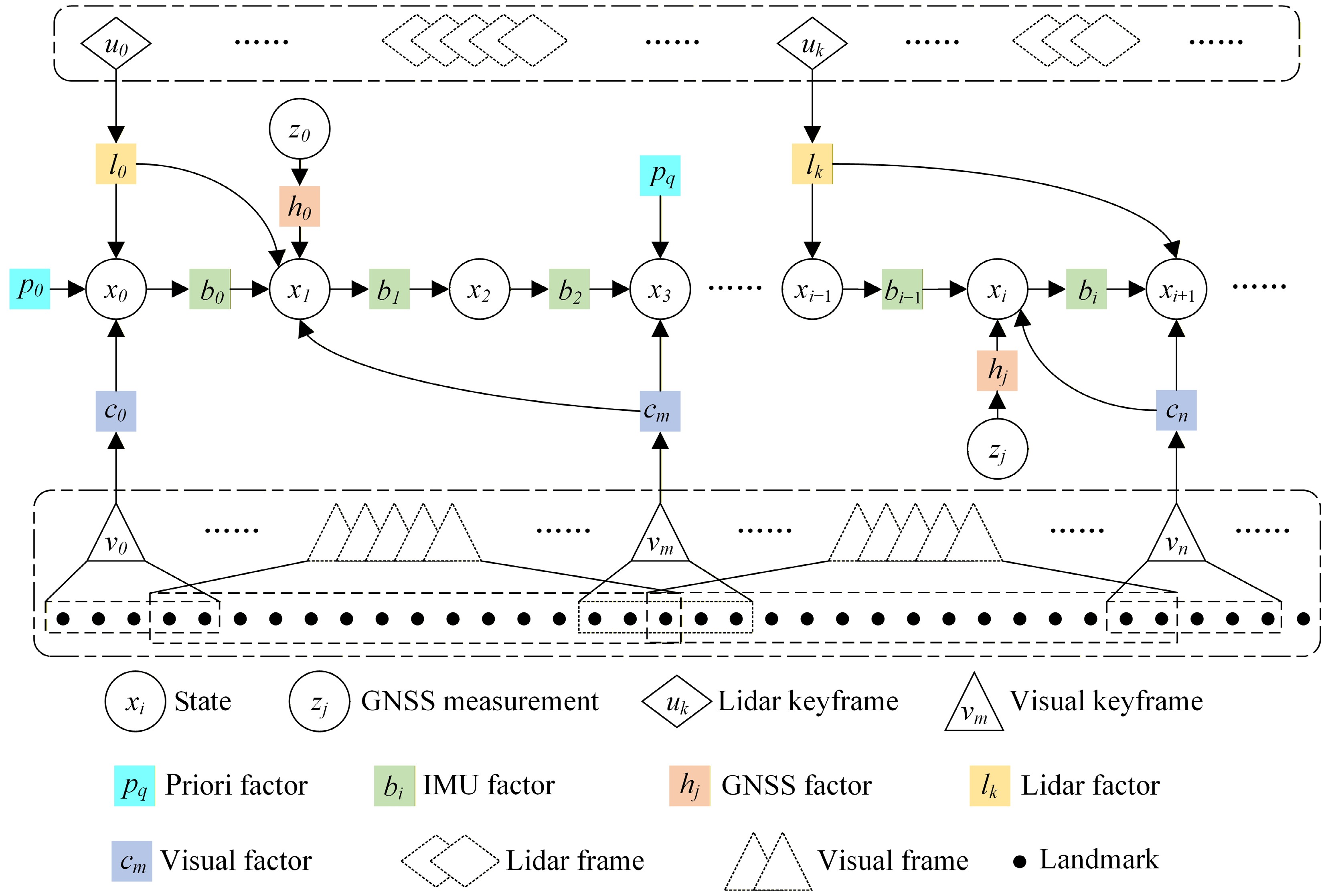
Figure 4. 

Factor graph optimization framework.

The full state vector X contains the navigation states x_i in the sliding window, the camera and LiDAR spatio-temporal parameters x_cam and x_lidar, and the inverse depths of visual features λ_i:

The state estimation problem is formulated as a Maximum A Posteriori (MAP) estimation problem, which is solved by minimizing the prior term and the Mahalanobis norms of all measurement residuals^[22]. Based on the sensor models derived above, the objective function includes the priori constraint, IMU pre-integration constraint, visual reprojection constraint, LiDAR point-surface geometric constraint, and GNSS position constraint:

Each of them corresponds to the a priori factor, IMU pre-integration factor, visual reprojection factor, LiDAR point-to-plane factor, and GNSS position factor, respectively. Their weights are determined by the information matrices. Here, the information matrix represents the inverse covariance of the corresponding residual and reflects the confidence of each measurement factor. The objective function jointly estimates the pose, sensor extrinsic parameters, and temporal offsets of the camera and LiDAR. During operation, new keyframes are added to the sliding window, and old states are marginalized to keep the problem size bounded. To avoid losing historical constraints, the related information of the removed frame is converted into a prior factor through the Schur complement and passed to the current window. This mechanism preserves historical information while limiting the optimization scale.

To examine the local observability of the online spatio-temporal calibration parameters, the linearized factor graph is analyzed in each sliding window. The optimized state is divided into the navigation state x, the calibration parameters θ, and the visual feature inverse depths λ. After linearization, the residual is expressed as:

where, J_x, J_θ, and J_λ are the corresponding Jacobian matrices of the residual with respect to these variables. By marginalizing the accompanying variables η = [x; λ], the marginal information matrix of θ is obtained by the Schur complement:

The rank and minimum eigenvalue of $ \boldsymbol{\boldsymbol{\Lambda}}_{\theta} $ are used as local observability indicators. Weak observability may occur under low-dynamic motion, nearly straight-line motion, insufficient visual parallax, or LiDAR geometric degeneracy.

Ceres Solver is used as the nonlinear optimization engine, and the Levenberg–Marquardt (LM) algorithm is adopted to solve the above cost function iteratively. In each iteration, the Jacobian matrix of the residual term with respect to the state variable needs to be calculated. For rotation updates, a left-multiplicative quaternion error model is used in the tangent space to avoid singularities in orientation parameterization.

Elastic variable structure

To improve robustness under partial sensor degradation, an elastic variable-structure mechanism is introduced at the factor level. GNSS, visual, and LiDAR factors can be manually disabled according to sensor availability or automatically removed according to residual consistency. IMU pre-integration factors and marginalization priors are retained in all configurations to preserve motion propagation and historical constraints.

The automatic factor selection is based on the chi-square consistency test. For each residual factor, the rejection threshold is selected according to its residual dimension at the 0.99 confidence level. This avoids using a fixed threshold for different sensor modalities and reduces over-aggressive rejection of valid measurements. For GNSS observations, an inconsistent factor is directly removed, indicating that the corresponding GNSS observation is inactive at that timestamp. For visual and LiDAR measurements, isolated inconsistent factors are first removed at the feature level. Frame-level modality degradation is declared only when more than 50% of the factors in that frame are rejected, which helps distinguish isolated outliers from temporary sensor-level degradation.

According to the remaining active factors, the estimator can operate under LVIG, LVI, VIG, LIG, VI, and LI topologies, where L, V, I, and G denote LiDAR, visual, IMU, and GNSS factors, respectively. During topology switching, only the parameter blocks constrained by the remaining active factors are effectively updated. The navigation states and IMU biases are retained in all topologies. If visual factors of a frame are removed, the corresponding reprojection residuals and inverse-depth variables are excluded, while the camera-related spatio-temporal parameters are maintained by previous estimates. Similarly, if LiDAR factors are removed, the LiDAR-related extrinsic and temporal-offset parameters are not updated by that frame. Removing a GNSS factor only disables the global position constraint at the corresponding timestamp.

The active topology is determined by the remaining valid factors after sensor-availability checking or residual-consistency-based factor culling. Based on this criterion, the elastic topology adjustment is embedded into a two-stage sliding-window optimization process, as summarized in Algorithm 1.

The active topology is determined by the remaining valid factors in the sliding-window graph. The proposed mechanism is a practical factor-level topology adjustment strategy rather than a formal global convergence guarantee under arbitrary sensor failures. During topology switching, the estimator is not reinitialized; instead, IMU pre-integration factors and marginalization priors are retained to maintain temporal continuity. The practical stability of this process is evaluated in the topology-switching robustness analysis.

The experiments were conducted on two public multi-sensor datasets with different platform characteristics. The i2Nav-Robot dataset^[23] was used to evaluate long-distance trajectory accuracy and robustness in urban ground-platform scenarios. Four types of sensor measurements were used in the experiment, including IMU, GNSS, camera, and LiDAR. In the i2Nav-Robot dataset, the IMU data were collected by an ADIS16465 IMU, the GNSS observations were provided by an OEM719 receiver, the visual measurements were obtained from the left camera of an AVT Mako-G234 camera, and the LiDAR point clouds were collected by a Hesai AT128 LiDAR. The NTU VIRAL dataset^[24] was used to evaluate the cross-platform applicability of the proposed framework on an MAV platform. Since this dataset does not provide GNSS observations, three types of sensor measurements were used in the MAV experiment. The IMU data were collected by a VectorNav VN100 IMU, the LiDAR point clouds were collected by an Ouster OS1-16 LiDAR, and the visual measurements were obtained from a uEye 1221 LE camera.

All experiments were performed on a laptop equipped with an AMD Ryzen 7 7745HX processor with 8 physical central processing unit (CPU) cores and 16 logical processors, and 16 GB of random access memory (RAM). The software environment was Ubuntu 20.04 with Robot Operating System (ROS) Noetic, and Ceres Solver was used for nonlinear optimization. The estimated trajectories were evaluated using the evo evaluation tool, a Python package for the evaluation of odometry and SLAM, after alignment with the reference trajectories. The main metrics include absolute translation error (ATE) and absolute rotation error (ARE), which are computed as follows:

where, t_e,i and t_g,i denote the estimated and reference position vectors at timestamp i, respectively; R_e,i and R_g,i denote the corresponding estimated and reference rotation matrices; ||·||₂ is the Euclidean norm; tr(·) is the matrix trace; and e_t,i and e_r,i represent the translational and rotational absolute pose errors. The pose error at timestamp i is regarded as the absolute pose error (APE), whose translational and rotational components are given by e_t,i and e_r,i. The reported ATE and ARE values are computed as the root mean square errors (RMSE) of e_t,i and e_r,i over all timestamps, respectively.

Ground mobile platform experiment

Trajectory estimation accuracy analysis

Through the qualitative and quantitative evaluation of the operation results of the ground mobile platform in the complex road environment, the long-distance trajectory accuracy of the proposed factor-graph framework is evaluated. The experimental data is derived from the building00 sequence of the i2Nav-Robot dataset. The total length of the sequence is 1,672 m, and the running time lasts 1,200 s. It covers a variety of challenging scenes such as high-rise buildings and building overhead layers with alternating strong and weak light.

The computational cost was evaluated by the backend optimization time per sliding window rather than by single-frame processing time, because one window contains visual, LiDAR, GNSS, and IMU factors. In all experiments, the sliding-window size was fixed to 20 keyframes. With this setting, the average backend optimization time was 28 ms, the average CPU resource utilization was approximately 27% of the total logical-processor capacity, and the peak memory usage was about 1.2 GB. A larger sliding window generally increases the backend optimization time and correction-update latency. However, this latency mainly affects the backend state correction, while the high-frequency pose output is still propagated in real time by IMU prediction and corrected after each optimization window.

The proposed multi-source fusion navigation system is named VILOG, referring to a Visual-Inertial-LiDAR odometry system with GNSS constraints. It integrates visual, inertial, LiDAR, and GNSS measurements for pose estimation. For comparison, representative open-source frameworks in the sensor-fusion field are selected, including the classic visual inertial odometer VINS-Mono^[3], the high-performance LiDAR inertial odometer Fast-LIO2^[6], and the LiDAR-enhanced visual inertial fusion system LE-VINS^[11]. The trajectory pairs of different algorithms after global alignment are shown in Fig. 5.

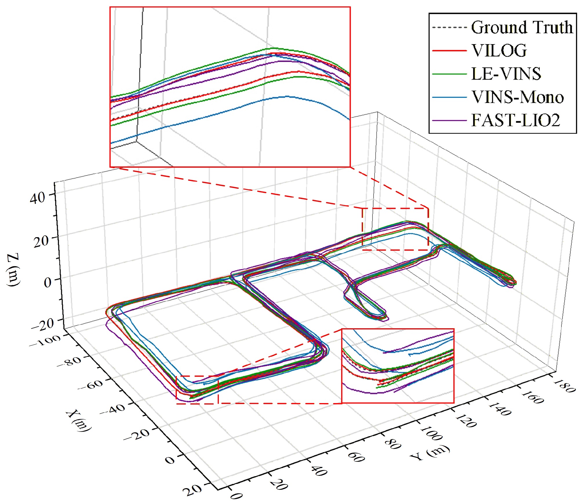
Figure 5. 

Trajectory comparison of different algorithms.

From the perspective of qualitative trajectory performance, VINS-Mono and FAST-LIO2 showed obvious cumulative drift during long-distance operation. It can be seen from the enlarged regions of the starting point and the end point that there is a significant spatial offset between the trajectories generated by these two algorithms and the true values, which cannot maintain the consistency of the global scale. In terms of local details and dynamic robustness, although LE-VINS performs well in the straight line segment, the estimation accuracy decreases during steering, and the trajectory has a large error. In contrast, the VILOG trajectory remains closer to the reference trajectory over the tested sequence, especially in the steering area with unstable features due to dramatic changes in the angle of view; it still maintains smooth and accurate tracking.

In order to further quantify the positioning ability of the algorithm, the ATE and ARE of each algorithm under the building00 sequence are calculated. The specific quantitative comparison data are shown in Table 1.

Through quantitative analysis, it can be seen that the algorithm achieves the best accuracy performance in the test sequence. In the urban scene of several kilometers, the ATE of VILOG is only 0.18 m. Compared with FAST-LIO2 of 1.90 m and VINS-Mono of 3.82 m, the accuracy of VILOG is improved by an order of magnitude. At the same time, in the ARE dimension, VILOG also performs best, and is as low as 0.21°, which is superior to other fusion algorithms. The data comparison proves that VILOG has achieved the minimum absolute pose error in the two key dimensions of translation and rotation, and its overall positioning ability is better than the current mainstream fusion navigation algorithm.

Figure 6 shows the curve of the ATE of each algorithm over time during the 1,200 s of operation. The errors of VINS-Mono and FAST-LIO2 show larger fluctuations, and the maximum error once exceeds 5 m, reflecting that pure VIO or LIO is easily affected by environmental degradation and cumulative drift in complex long-distance motion. In contrast, the VILOG error curve is controlled within 0.5 m; not only is the overall value much lower than the comparison algorithm, but it also shows convergence stability throughout the process. Even in the period of accuracy fluctuation of LE-VINS, VILOG still maintains a stable and consistent low error output.

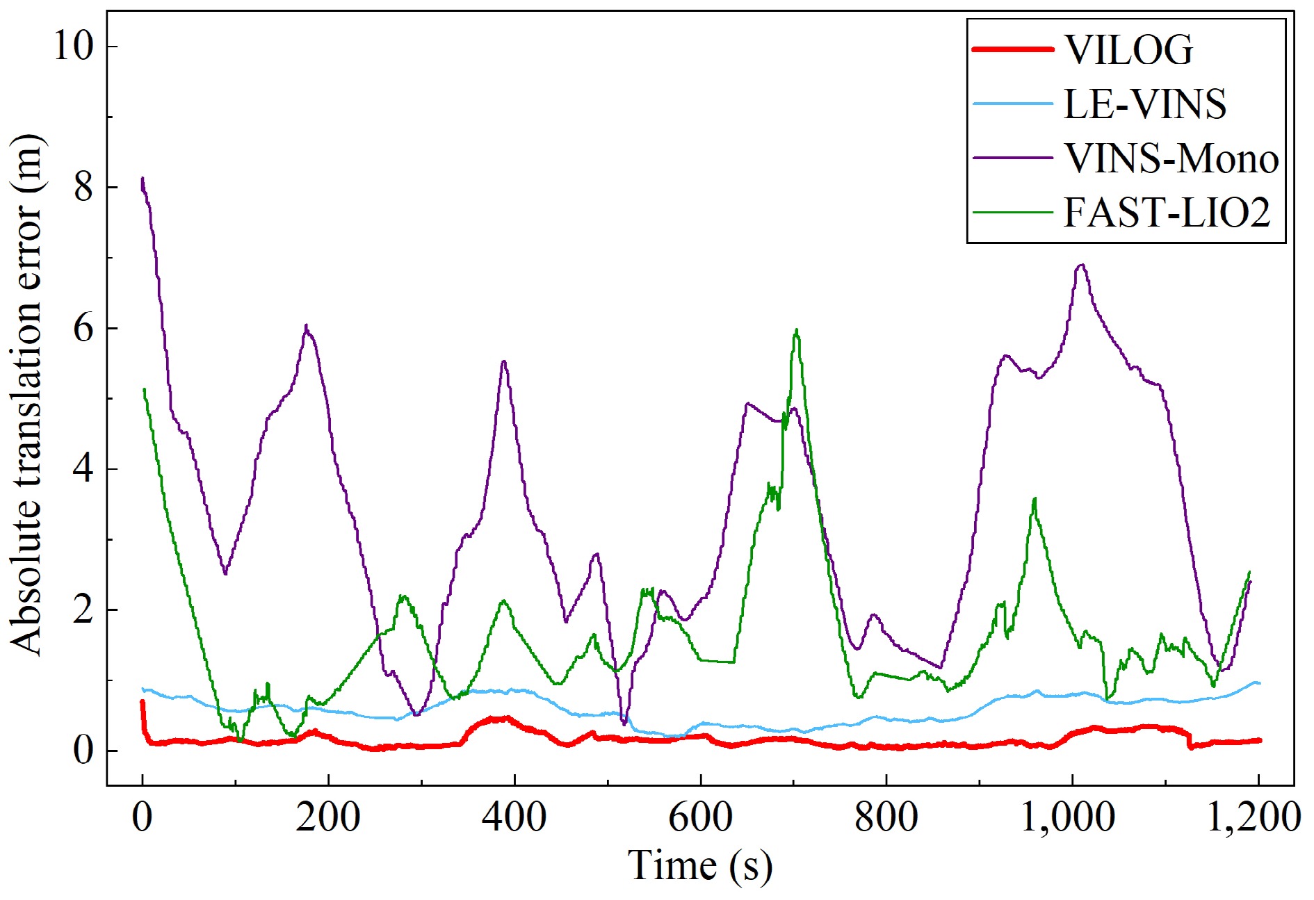
Figure 6. 

ATE variation curve.

Online spatio-temporal calibration behavior

This section evaluates the online refinement behavior of the camera-IMU and LiDAR-IMU spatio-temporal parameters during motion. In the experiment, the parameters are given an initial guess value, and the observation optimizer uses the geometric consistency of multi-source observations to make the parameters converge.

Aiming at the online estimation of spatial extrinsic parameters, the system uses LiDAR point-surface features and visual reprojection residuals to adjust the pose transformation matrix in real time. The real-time calibration curve of the camera and LiDAR extrinsic parameters during the operation of the program is shown in Fig. 7.

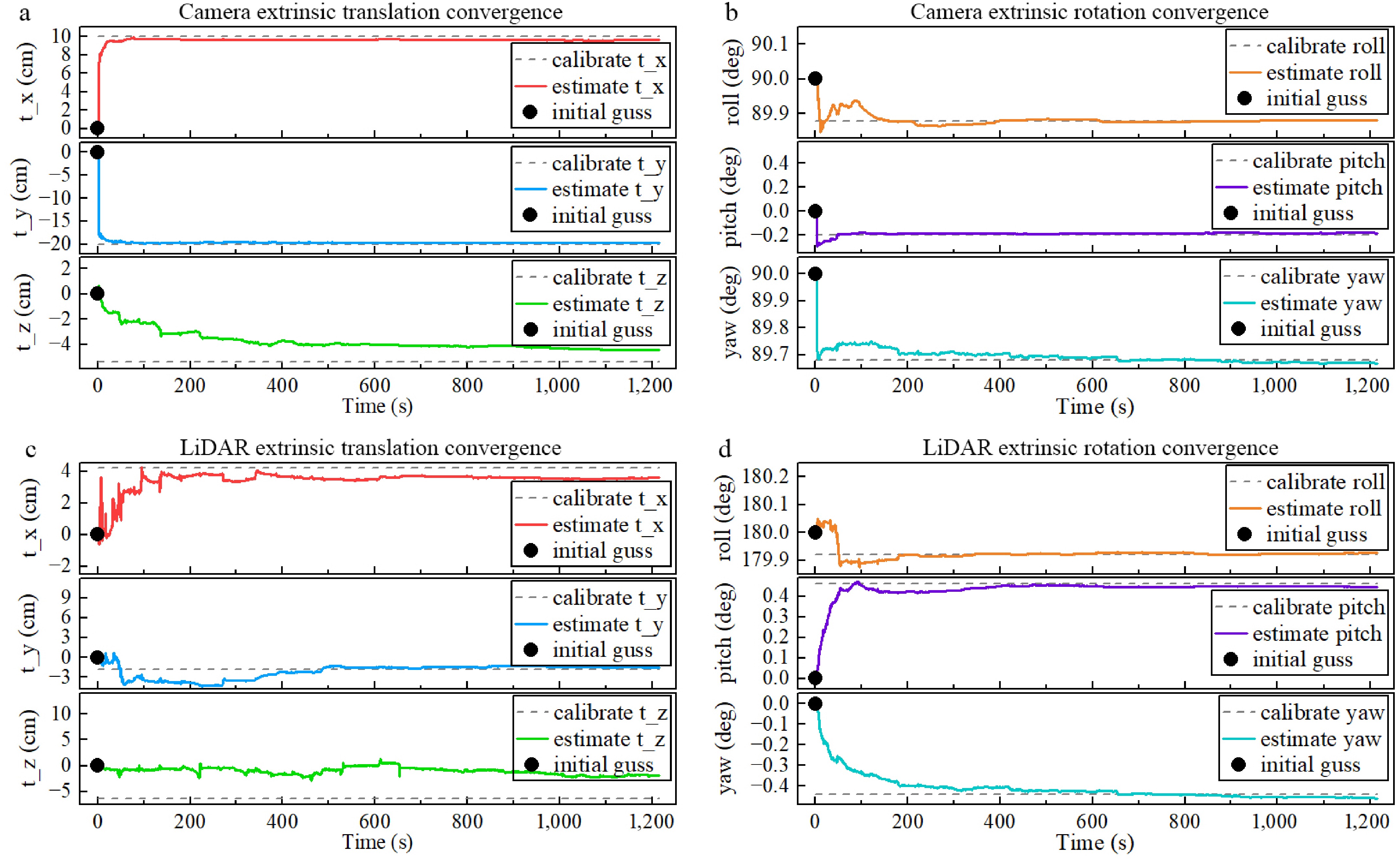
Figure 7. 

Real-time calibration of camera and LiDAR extrinsic parameters.

The extrinsic parameters are initialized with rough values based on the physical installation. As the system enters the rich motion area of multi-source observation, each component parameter shows good convergence characteristics. For the camera extrinsic parameter estimation Fig. 7a and b, the core optimization variables are quickly adjusted within the first 200 s of operation, and finally stabilized near the calibration reference provided by the dataset. For LiDAR extrinsic parameter estimation in Fig. 7c and d, although the point cloud registration residual has a small oscillation in the initial stage, the multi-frame geometric constraints reduce the deviation from the initial guess, and the rotation and translation components approach the dataset calibration reference.

The online estimation results of the camera-IMU and LiDAR-IMU temporal offsets are shown in Fig. 8. The curves denoted as 'base' correspond to the raw dataset without any manually introduced timestamp offset. Starting from zero initial values, both temporal offsets are gradually constrained by the time-delay compensation model in the factor graph and converge to stable values. In this evaluation, the estimates after the first 100 s are regarded as the converged stage, and the mean values over this interval are used for quantitative analysis. As shown in Fig. 8a, the camera temporal offset converges rapidly in the early stage and then remains around a mean value of 2.21 ms after convergence, with small fluctuations caused by variations in visual feature tracking quality. Fig. 8b shows that the LiDAR temporal offset also becomes stable after the initial adjustment, with a converged mean value of approximately 0.35 ms. These results indicate that the introduced temporal parameters can be effectively constrained by the multi-source residuals during online optimization.

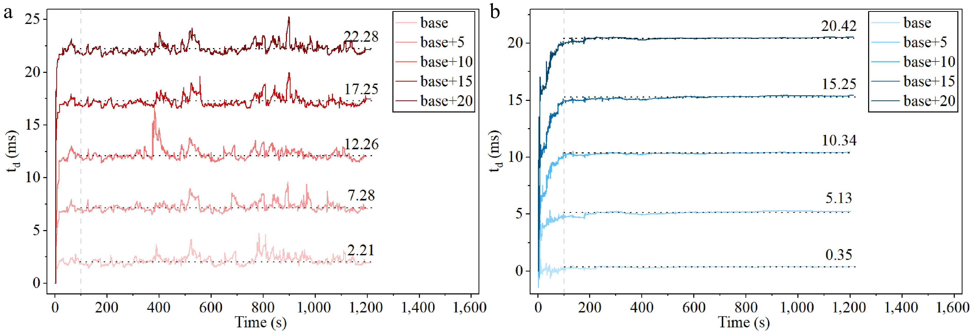
Figure 8. 

Online estimation of camera-IMU and LiDAR-IMU temporal offsets.

However, since the i2Nav-Robot dataset does not provide calibrated ground-truth temporal offsets, the base curves in Fig. 8 cannot alone verify the absolute accuracy of the estimated time delays. To further evaluate the effectiveness of the proposed online temporal calibration method, known timestamp increments of 5, 10, 15, and 20 ms were manually introduced into the camera and LiDAR measurements, and the corresponding estimation results are also plotted in Fig. 8. The estimates after the first 100 s were used to compute the mean, median, and RMSE of the recovered increments, as summarized in Table 2. For the camera temporal offset, the estimated increments are 4.79, 10.00, 14.90, and 20.08 ms for the four injected increments, with RMSE values below 0.24 ms. For the LiDAR temporal offset, the estimated increments are 5.08, 10.05, 15.04, and 20.07 ms, with RMSE values of about 0.43–0.52 ms. These results show that the proposed method can accurately recover known relative temporal-offset increments after convergence, thereby validating the accuracy and reliability of the proposed online temporal calibration method.

Topology-switching robustness analysis

This section evaluates the topology-switching capability of the proposed elastic factor management mechanism under reduced sensor configurations and dynamic sensor loss-recovery settings. In the static configuration experiment, the corresponding visual, LiDAR, or GNSS factors were manually disabled before optimization to simulate different active topologies. Figure 9 shows the ATE distribution of different sensor combinations when running the same sequence building00. The experimental results show that with the decrease in the number of fusion sensors, although the distribution interval of the positioning error of the system has a certain degree of expansion, the median and distribution range indicate that the estimator maintains trajectory tracking under reduced sensor configurations, and no obvious trajectory divergence is observed.

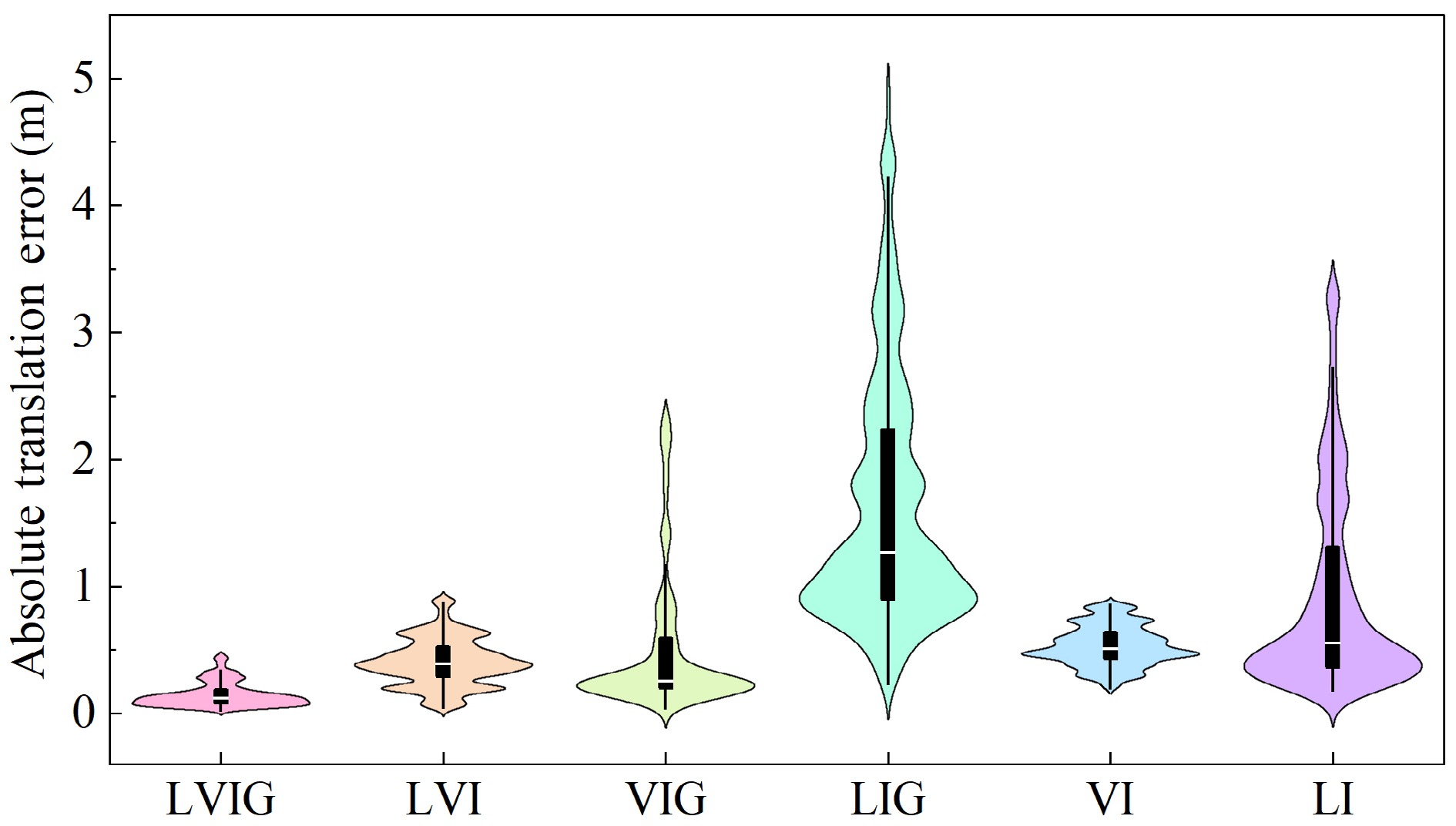
Figure 9. 

ATE distribution of different sensor combinations.

Figure 10 further evaluates the response of the estimator when selected sensor factors are disabled and then restored during operation. The loss and recovery intervals are predefined to evaluate the estimator continuity under controlled topology changes. This experiment focuses on the continuity of state estimation during topology switching, rather than on the completeness of sensor-fault diagnosis. The red curve records the error fluctuation of the system in the process of GNSS, visual, LiDAR loss, and recovery. When a certain observation mode is missing, the ATE will rise in stages due to the weakening of constraints, but after the sensor provides effective constraints again, the error can be reduced to a low level. At the switching moments, no obvious pose jump or trajectory divergence is observed in the error curve. The results indicate that the elastic topology-switching can maintain continuous pose estimation during the tested sensor loss-and-recovery process, although the estimation error increases when observation constraints are reduced.

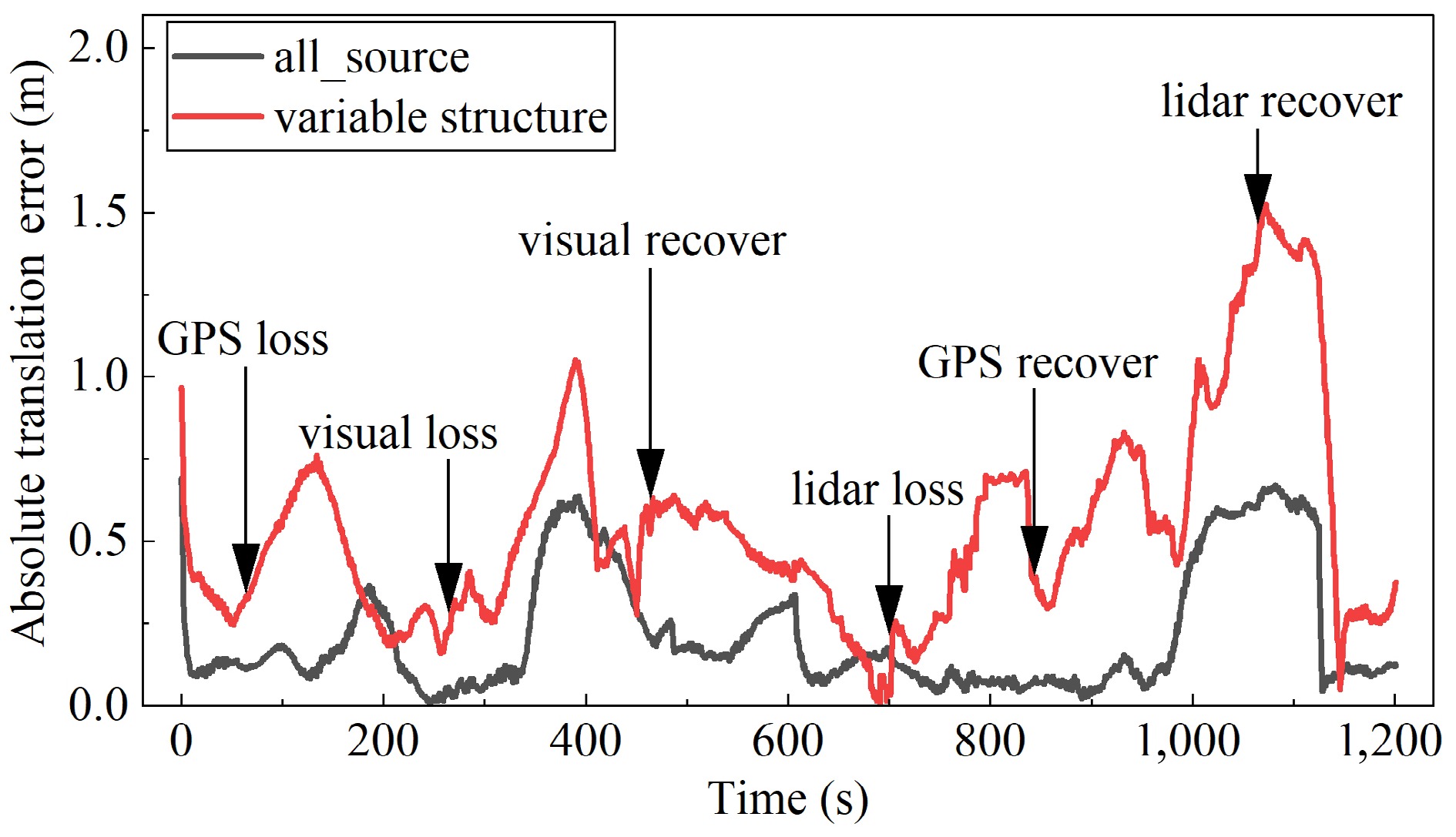
Figure 10. 

ATE changes during sensor loss and recovery.

Expansion experiment of the MAV platform

This section aims to verify the scene migration ability of the VILOG multi-source fusion scheme for different dynamic carriers and motion dimensions. The core advantage of the system is that the manifold-based factor graph optimization framework has good versatility, and the construction of its state vector and residual model is completely based on the general rigid body kinematics description in three-dimensional space. When migrating from the ground platform to the high-maneuverability MAV platform, there is no need to reconstruct the core algorithm logic. It is only necessary to update the initial spatial extrinsic parameters between the camera, LiDAR, and IMU according to the physical structure of the MAV, and adjust the data noise distribution parameters according to the sampling specifications of the sensor. The system can be used for high-dynamic three-dimensional six-degree-of-freedom motion estimation.

Figure 11a is the three-dimensional trajectory calculation result of VILOG under the eee_03 sequence of the Unmanned Aerial Vehicle (UAV) dataset NTU VIRAL, which contains typical aircraft ascending, descending, and rotating motion scenes. The experimental results show that the estimated trajectory generated by VILOG is consistent with the real reference trajectory in three-dimensional space, and the system captures the motion details caused by MAV steering and height changes. Figure 11b shows that the ATE is always below 0.8 m during a test period of about 150 s, and there is no tracking failure point in the complex flight motion. These results provide preliminary evidence of the cross-platform applicability of the proposed framework under MAV motion.

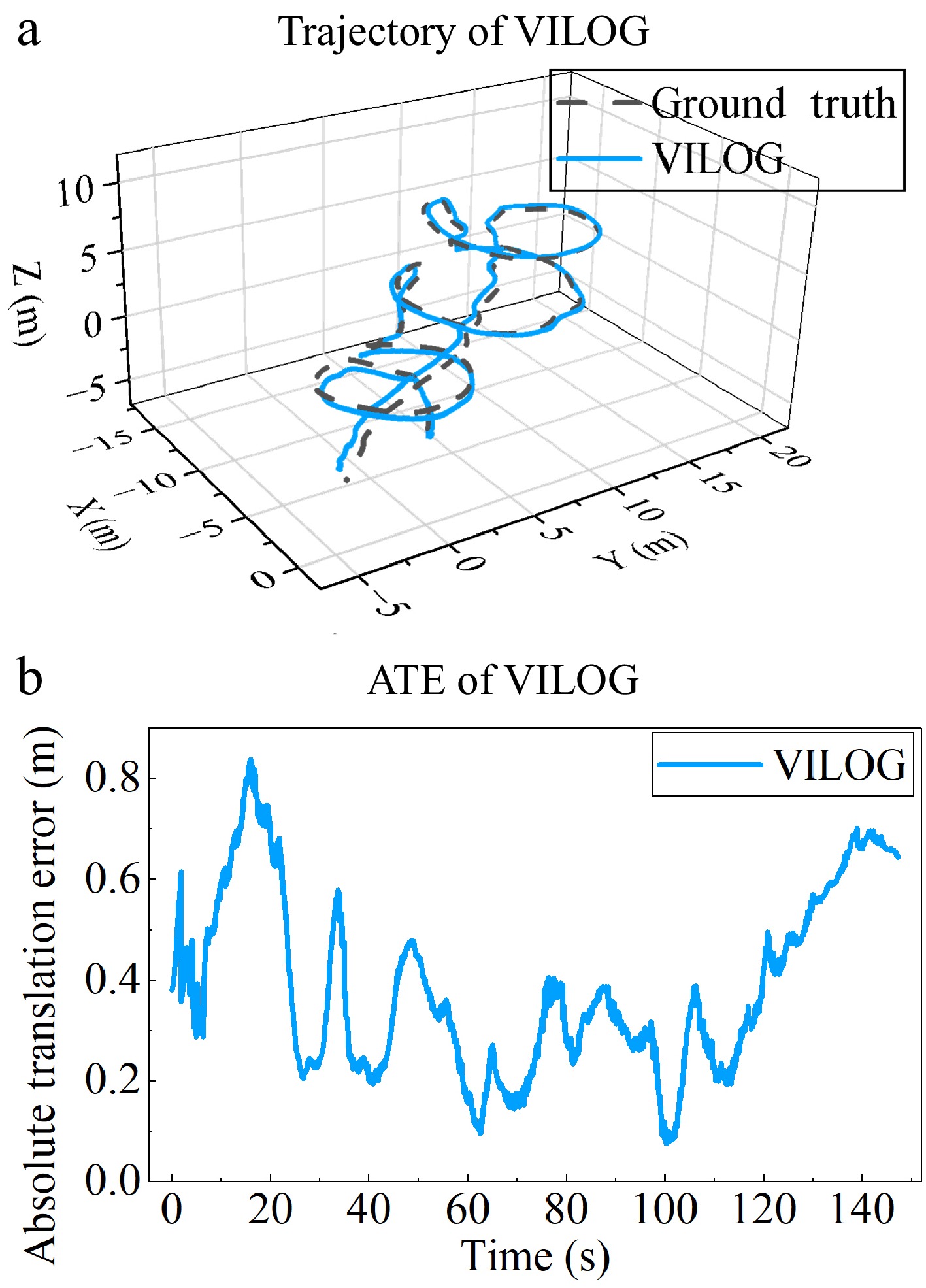
Figure 11. 

Multi-source fusion navigation effect of MAV platform.

The experimental results show that the proposed factor-graph-based multi-source fusion framework improves trajectory accuracy on the tested ground mobile platform sequence. Compared with VINS-Mono and FAST-LIO2, VILOG benefits from the joint use of visual, LiDAR, inertial, and GNSS constraints, which helps reduce cumulative drift in long-distance operation. Compared with LE-VINS, the additional GNSS global position factor provides an absolute constraint for trajectory correction. These results indicate the benefit of jointly optimizing local relative constraints and global position observations in the same sliding-window framework.

The online spatio-temporal calibration results indicate that the camera-IMU and LiDAR-IMU extrinsic parameters can be refined from rough initial values and converge to stable ranges close to the dataset-provided calibration references. The temporal-offset estimation results exhibit stable convergence. Furthermore, the injected timestamp-increment experiments demonstrate that the proposed method can accurately recover known temporal-offset increments with low RMSE, providing quantitative evidence for the effectiveness of the online temporal calibration. In addition, the sensor-combination and loss-recovery experiments show that the estimator can maintain continuous pose output under reduced sensor configurations. When GNSS, visual, or LiDAR factors are removed, the estimation error increases due to the reduction of active constraints; when these factors are restored, the error decreases again. No obvious trajectory divergence or abrupt pose jump is observed during the tested topology-switching process.

Compared with existing tightly coupled multi-sensor navigation systems, the contribution of this work is not to claim a completely new fusion paradigm, but to integrate several practical functions within a unified factor-graph framework. The proposed framework combines local visual-LiDAR-inertial constraints and GNSS global position observations, introduces online spatio-temporal calibration for heterogeneous sensors, and supports factor-level topology adjustment under partial sensor degradation. This design is practically useful for robotic mobile platforms, especially MAV-oriented applications where GNSS degradation, visual texture loss, LiDAR geometric weakness, and inertial drift may occur alternately during operation.

Although the experimental results demonstrate the effectiveness of the proposed framework on the tested datasets, more effective sensor-degradation assessment and fault-detection strategies are still needed to further improve its applicability in practical onboard scenarios.

This paper proposed an elastic multi-source fusion navigation framework based on factor graph optimization. The framework incorporates IMU pre-integration, visual reprojection, LiDAR point-to-plane, and GNSS global position factors into a unified sliding-window optimization problem. Camera-IMU and LiDAR-IMU extrinsic parameters and temporal offsets are included in the state vector to support online spatio-temporal refinement. In addition, a residual-consistency-based elastic factor management strategy is introduced to suppress inconsistent measurement factors and support active topology adjustment under partial sensor degradation.

Experiments on an urban ground mobile platform dataset and an MAV dataset show that the proposed method improves trajectory accuracy on the tested sequences, exhibits stable online calibration behavior, and maintains continuous pose output during sensor loss and recovery. The runtime results also indicate that the framework can support online state updating on the evaluated computing platform. Future work will focus on more effective sensor-degradation assessment, fault-detection strategies, and lightweight onboard implementation to further enhance the applicability of the proposed system in practical onboard scenarios.