Enhanced indoor UAV UWB localization algorithm based on outlier removal and an improved iterative ensemble Kalman filter

Indoor inspection, warehouse automation, and autonomous aerial robotics have created increasing demand for localization methods that can operate without stable GNSS support. In urban canyons and indoor spaces, GNSS signals are often unavailable or severely degraded because of multipath reflections, signal blockage, and NLOS conditions^[1]. In such scenarios, UAVs cannot rely on satellite positioning to obtain stable and accurate position information, which creates a critical challenge for autonomous navigation, hovering control, inspection, and cooperative operation. To overcome this limitation, various indoor positioning technologies have been developed, including WiFi^[2], Bluetooth Low Energy^[3], visual odometry^[4], and pure inertial navigation^[5]. Nevertheless, these methods still involve trade-offs among localization accuracy, spatial coverage, environmental dependence, and real-time responsiveness. By contrast, UWB ranging offers subnanosecond pulse intervals and picosecond-level time resolution, enabling centimeter-level ranging precision and supporting high-efficiency positioning sensor networks^[6]. Therefore, UWB has become a promising technology for indoor UAV localization.

In a typical indoor UWB deployment, anchors are installed at known positions, while the UAV carries an onboard UWB tag. By measuring the propagation time or time difference of wireless pulses between the anchors and the tag, the UAV position can be estimated using trilateration or TOA/TDOA-based localization algorithms^[7]. In general, at least three anchors are required for two-dimensional localization, and four or more anchors are commonly used to improve geometric robustness and localization reliability. However, practical indoor UWB signals are easily affected by attenuation, reflection, and multipath propagation. These effects may introduce decimeter- or even meter-level ranging errors and generate abnormal observations that significantly degrade localization accuracy^[8]. Moreover, many classical localization methods are derived under Gaussian-noise assumptions and have limited adaptability to complex and time-varying indoor channel conditions^[9]. Therefore, improving the robustness and accuracy of UWB-based indoor UAV localization remains an important research problem.

To improve UWB localization reliability, outlier removal is usually required before recursive state estimation because the final positioning result is directly affected by the quality of the ranging measurements. Existing outlier suppression methods can generally be divided into classical filtering-based approaches and machine-learning-based approaches. Traditional filters, such as Gaussian smoothing^[10], median filtering^[11], and moving average filtering^[12], perform basic anomaly suppression by smoothing the raw range sequence or discarding samples that exceed predefined thresholds. However, these methods usually rely on relatively strong statistical assumptions and can be ineffective when the measurements contain bursty, clustered, or irregular outliers. In such cases, they may either fail to remove severe abnormal observations or mistakenly reject valid measurements. Recent studies have also explored deep-learning-based solutions. For example, Jiang et al.^[13] employed a convolutional neural network to classify and denoise channel impulse responses, and Nguyen et al.^[14] investigated deep-learning-based UWB localization. Although these methods are promising, they typically require substantial computational resources, which limits their deployment on UAV platforms and embedded systems with strict onboard processing constraints.

Ranging-level outlier suppression improves the input quality of UWB localization, but it does not by itself solve the complete state-estimation problem. After preprocessing, the localization backend still has to transform nonlinear multi-anchor range observations into a temporally consistent UAV state estimate while coping with residual abnormal measurements, channel-dependent uncertainty, and time-varying motion disturbances. Correspondingly, the development of UWB localization algorithms has gradually evolved from pure geometric solvers toward more robust state-estimation frameworks. The classical trilateration method is intuitive and easy to implement, but it is highly sensitive to ranging noise and anchor geometry^[15]. Linearized or differential least-squares methods reduce computational complexity, but they neglect higher-order nonlinear error terms and may become unreliable under poor geometric configurations or strong noise contamination^[16]. Chan & Ho's two-stage closed-form method provides an efficient weighted least-squares initial estimate^[17], and the Levenberg–Marquardt variant can further reduce residual errors through iterative refinement^[18]. However, these static localization approaches mainly rely on instantaneous measurements and cannot exploit motion continuity for recursive prediction and smoothing.

Kalman-filter-based methods address this temporal estimation requirement by combining motion models and ranging observations in a recursive prediction-and-update framework^[19,20]. Among them, the ensemble Kalman filter (EnKF) provides a sample-based approximation of the state distribution and avoids explicit Jacobian linearization, which makes it attractive for nonlinear state-estimation problems such as range-based UWB localization^[21]. However, the standard EnKF still depends on fixed process and measurement covariance settings, and its performance can be affected by finite ensemble sampling errors, residual ranging outliers, and strong nonlinear measurement responses. These limitations become more evident in indoor UWB localization, where different anchor channels may exhibit nonuniform reliability due to NLOS propagation, multipath reflection, and dynamic occlusion.

To improve the robustness of ensemble-based nonlinear filtering, iterative EnKF and adaptive EnKF variants have been investigated in recent studies. Sakov et al.^[22] generalized the iterative ensemble Kalman filter to imperfect-model cases with additive model error, showing that iterative ensemble analysis can improve nonlinear filtering performance. Berry & Sauer^[23] developed an adaptive EnKF framework for nonlinear systems, in which covariance adaptation is used to compensate for model and observation uncertainty. Raanes et al.^[24] further studied adaptive covariance inflation in the EnKF and discussed its role in mitigating sampling and model-error effects. In addition, Tao et al.^[25] proposed a maximum-correntropy ensemble Kalman filter to reduce the influence of non-Gaussian observation noise and large outliers. These studies provide important foundations for robust and adaptive ensemble filtering, but they are generally formulated as generic state-estimation methods and do not explicitly exploit the multi-anchor, channel-dependent abnormal ranging characteristics of indoor UWB localization.

For UWB positioning, recent robust and adaptive Kalman-filter-based methods have also been reported. For example, Zhao et al.^[26] combined unscented Kalman filtering with a maximum-correntropy criterion to reduce the influence of non-Gaussian UWB ranging errors, while Dong et al.^[27] introduced a robust adaptive cubature Kalman filter to handle dynamic NLOS conditions, model mismatch, and measurement outliers. These methods demonstrate the necessity of robust/adaptive filtering for UWB localization. However, most existing methods mainly improve the backend filtering update, robust cost function, or covariance adaptation strategy. In contrast, the present study focuses on a UWB-specific two-stage robustness design: multi-channel range-level outlier suppression is first used to improve measurement reliability, and an improved IEnKF backend is then used to jointly perform innovation-driven process covariance adaptation, channel-aware measurement covariance construction, and damped iterative ensemble analysis. Therefore, the proposed method differs from generic 'Robust EnKF + Adaptive Covariance' strategies by jointly addressing measurement-level outlier suppression, anchor-dependent ranging reliability, time-varying motion uncertainty, and nonlinear range-update stability within a lightweight indoor UAV UWB localization pipeline.

To address the sensitivity of indoor UWB localization to abnormal measurements in non-stationary environments, as well as the performance degradation of conventional filters under time-varying disturbances, this paper proposes an indoor UWB localization algorithm that tightly integrates multi-channel UWB outlier removal with an improved iterative ensemble Kalman filter. The contribution boundary of this study is the design and validation of a robust UWB-only localization pipeline for planar indoor UAV motion; the work does not claim to solve full three-dimensional multi-sensor navigation. The main contributions are summarized as follows:

1. A multi-channel UWB outlier removal strategy based on local Tukey reweighting is developed to address bursty, clustered, and channel-dependent abnormal ranging observations before state estimation. This front-end module improves the reliability of the range inputs supplied to the localization backend.

2. An improved IEnKF-based backend is developed for multi-anchor UWB localization. Different from generic robust EnKF or adaptive covariance inflation methods, the proposed backend jointly incorporates innovation-driven adaptive process covariance adjustment, channel-aware measurement covariance construction, and damped iterative ensemble analysis. The adaptive process covariance responds to time-varying motion uncertainty, the channel-aware measurement covariance represents nonuniform ranging reliability across anchors, and the damped iterative update improves numerical stability under nonlinear UWB range observations.

3. A systematic experimental evaluation is provided to delineate the contribution of the proposed pipeline, including comparisons with EKF, UKF, EnKF, MCC-UKF, and RA-CKF, module-level and component-level ablation studies, and parameter sensitivity analysis. This evaluation verifies not only the overall accuracy improvement but also the necessity and relative influence of the front-end and back-end mechanisms.

The remainder of this paper is organized as follows. The problem formulation and the proposed localization method, including the front-end outlier removal strategy and the backend improved iterative ensemble Kalman filter, are presented first. The experimental settings and performance evaluation results are then reported, followed by a discussion of the advantages, practical applicability, and limitations of the proposed method. Finally, the conclusions and future work are presented.

Figure 1 illustrates the overall structure of the proposed robust indoor UWB localization framework. Following the style of a modular localization pipeline, the framework consists of two coordinated components: a multi-channel UWB outlier removal module for improving range reliability and an IEnKF localization backend for robust recursive state estimation.

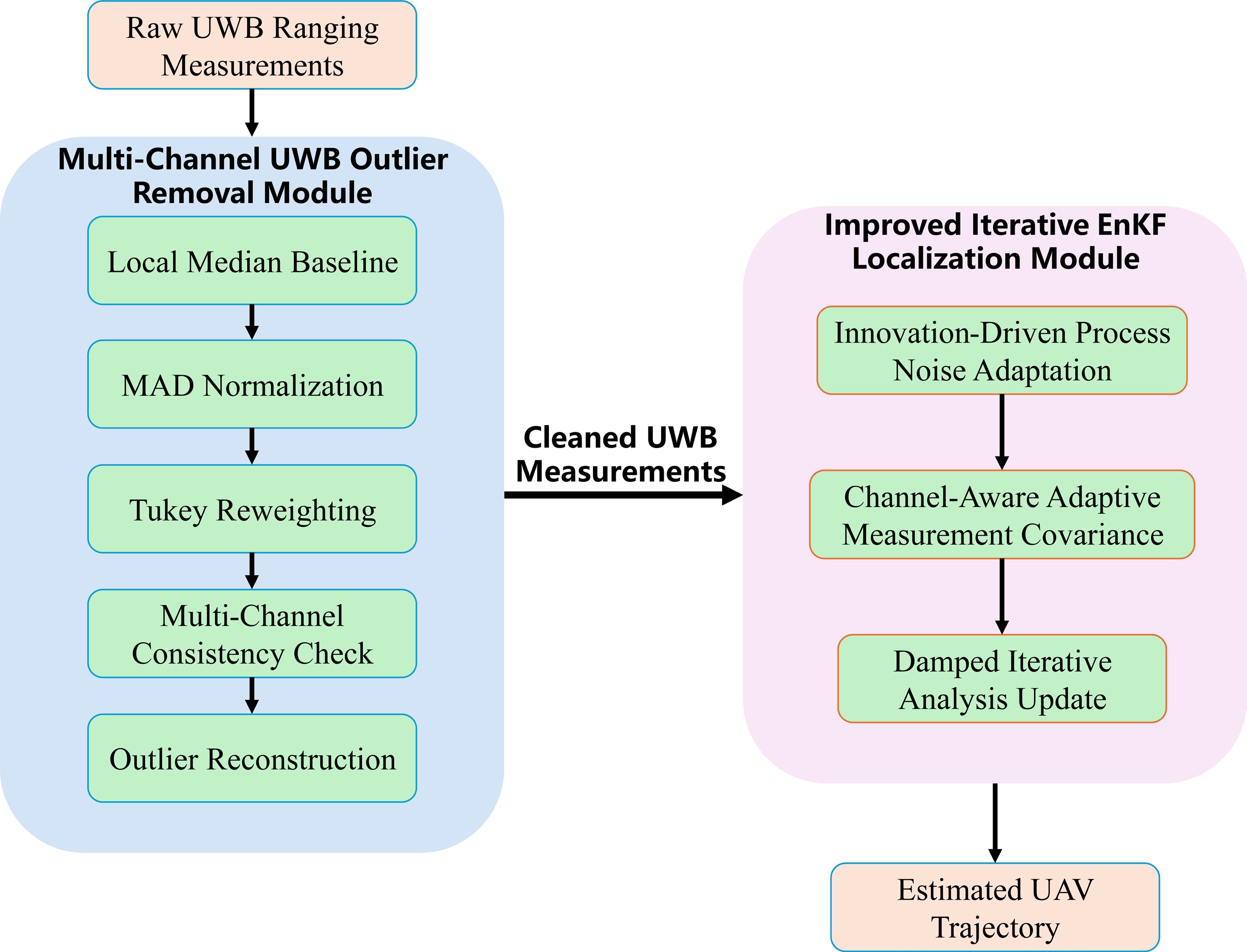
Figure 1. 

Structure of the proposed robust indoor UWB localization framework.

UAV dynamics and UWB measurement model

UAV dynamics model based on the constant-acceleration assumption

To support recursive state estimation for indoor UAV localization, the UAV is modeled as a point mass in a two-dimensional Cartesian coordinate system. Considering that low-speed indoor flight is generally smooth over short sampling intervals but may still exhibit local acceleration variations, a constant-acceleration model is adopted to describe its state evolution. Because the present experiments focus on horizontal indoor localization, only planar motion in the $ x $–$ y $ plane is considered.

We define the state vector at time step $ k $ as:

where, $ x_k $ and $ y_k $ denote the horizontal position of the UAV, $ (v_{x,k}, v_{y,k}) $ denote the velocity components, and $ (a_{x,k}, a_{y,k}) $ denote the acceleration components along the two coordinate axes.

Let the sampling interval be $ \Delta t $. Under the two-dimensional constant-acceleration model, the discrete-time state equation is written as:

where, $ {\boldsymbol{\eta}}_k $ denotes the discrete process noise and $ {\boldsymbol{Q}}_k $ is the corresponding process-noise covariance matrix. The state transition matrix is given by:

which assumes that the UAV acceleration remains approximately constant within each sampling interval, while unmodeled motion variations are absorbed into the process noise.

UWB ranging measurement model

Assume that $ m $ UWB anchors are deployed at known positions

At time step $ k $, the range measurement from the $ i $^th anchor to the UAV is modeled as:

where, $ v_{k,i} $ denotes the measurement noise associated with the $ i $^th anchor at time step $ k $.

By stacking all anchor-wise ranging observations, the UWB measurement vector can be written as:

Accordingly, the nonlinear measurement model is expressed as:

where,

and $ {\boldsymbol{R}}_k $ denotes the measurement-noise covariance matrix.

The initial two-dimensional position $ \hat{{\boldsymbol{p}}}_0=[\hat{x}_0,\hat{y}_0]^{T} $ is estimated from the first valid multi-anchor UWB ranging measurements using nonlinear least-squares multilateration:

The initial velocity and acceleration components are set to zero, and the initial covariance matrix is assigned as a diagonal matrix with relatively large entries to reflect initialization uncertainty.

Multi-channel UWB outlier removal algorithm based on local Tukey reweighting

Indoor UWB ranging observations are often affected by NLOS propagation, multipath interference, transient occlusion, and short-term environmental disturbances. These degradations may appear as isolated spikes, abnormal segments, or range jumps. Therefore, before recursive localization, local Tukey reweighting is used to improve the reliability of the range inputs supplied to the IEnKF backend.

Let the raw UWB ranging observations collected from $ m $ anchors over $ N $ sampling instants be organized into the matrix:

where, $ d_{k,i} $ denotes the ranging observation from anchor $ i $ at sampling instant $ k $, with $ i=1,2,\ldots,m $ and $ k=1,2,\ldots,N $.

For each anchor channel, a local median baseline is constructed within a sliding temporal window:

where, $ {\cal{N}}_{k,i} $ denotes the neighborhood samples of anchor/channel $ i $ within a window centered at time index $ k $.

The local fluctuation scale is estimated by the median absolute deviation:

A small lower bound is imposed on $ \sigma_{k,i} $ in implementation to avoid numerical instability.

Based on the local baseline and scale estimate, the normalized residual is defined as:

A Tukey-type reliability weight is introduced as:

where, $ c_{{\rm{T}}} $ is the Tukey cutoff parameter. Samples with large normalized residuals are assigned lower reliability weights, and severe local deviations are therefore prevented from dominating the subsequent range reconstruction.

To incorporate cross-channel consistency, a multi-channel abnormality indicator is defined as:

where, $ \tau_s $ is a soft threshold and $ \mathbb{I}(\cdot) $ is the indicator function. The final outlier decision for anchor/channel $ i $ at sampling instant $ k $ is given by:

where, $ \tau_m $ denotes the minimum number of simultaneously abnormal channels required to activate the multi-channel consistency rule, and $ \tau_r $ is a relaxed residual threshold under this condition.

To avoid removing physically plausible short-term range variations, a local trend check is introduced after residual-based screening. Let:

and

A suspicious sample is retained if its local variation trend remains consistent with that of the baseline within a prescribed tolerance. This step reduces the probability of removing valid samples during normal UAV motion.

For a confirmed abnormal segment, local interpolation based on neighboring valid samples is used for reconstruction. Let $ [s,e] $ denote a contiguous abnormal segment in anchor/channel $ i $. The reconstructed value is written as:

where, $ {\cal{I}}_{i}(k) $ denotes the interpolation result. The reconstructed value is then blended with the local median baseline:

where, $ \eta\in(0,1) $ 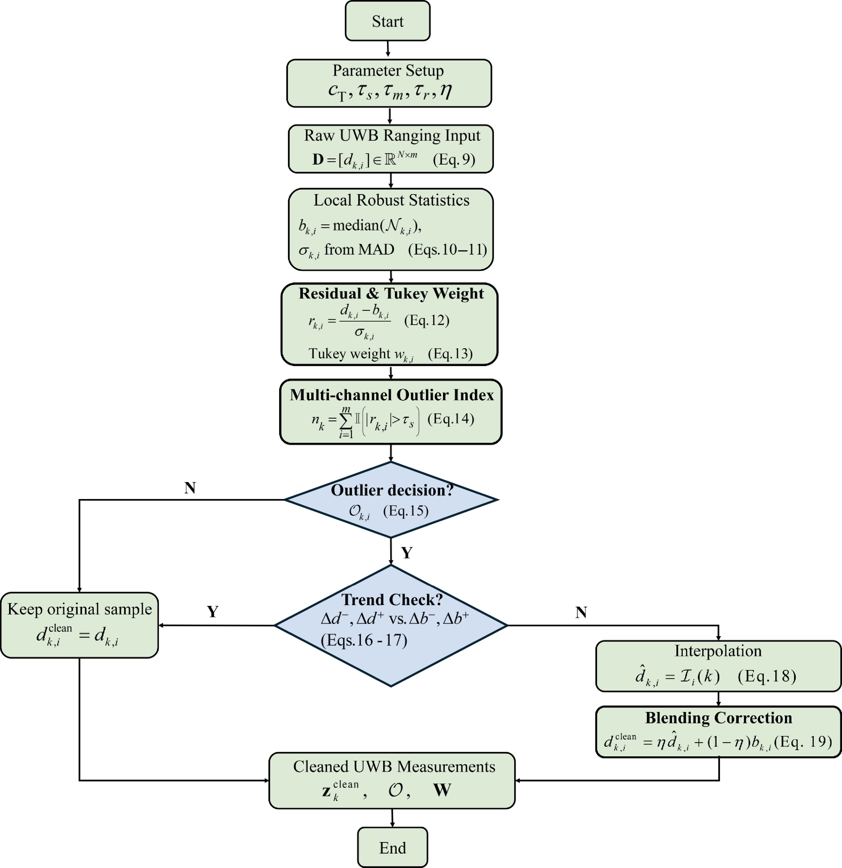is the blending coefficient. The resulting cleaned measurements are assembled into the corrected observation vector and used as the input to the subsequent adaptive IEnKF localization backend. The complete preprocessing workflow is summarized in Fig. 2.

Figure 2. 

Workflow of the proposed UWB outlier removal algorithm.

Because the centered window, forward-difference trend check, and segment-wise interpolation require future samples, the front-end module in this study is implemented as an offline or short-latency preprocessing procedure rather than a strictly causal online algorithm. For real-time deployment, it can be adapted using a backward sliding window and prediction-based or last-valid-sample replacement, while the backend IEnKF remains recursive and can operate online once preprocessed measurements are available.

UWB localization algorithm based on an improved iterative ensemble Kalman filter

After front-end outlier removal, the cleaned UWB ranging measurements are processed by the proposed IEnKF backend. The backend is designed to address three practical difficulties in indoor UWB localization: time-varying motion uncertainty, channel-dependent measurement inconsistency, and nonlinear range observation updates. Accordingly, it incorporates three coupled mechanisms, namely innovation-driven adaptive process covariance adjustment, channel-aware adaptive measurement covariance construction, and damped iterative ensemble analysis.

Based on the constant-acceleration motion model in Eq. (2) and the nonlinear UWB observation model in Eq. (6), the localization problem is written in the unified state-space form:

where, $ {\boldsymbol{x}}_{k} $ denotes the system state, $ {\boldsymbol{z}}_{k} $ denotes the UWB measurement vector, $ {\boldsymbol{f}}(\cdot) $ is the state transition function, and $ {\boldsymbol{h}}(\cdot) $ is the nonlinear observation function. The process noise and measurement noise are modeled as zero-mean Gaussian variables with covariances $ {\boldsymbol{Q}}_{k} $ and $ {\boldsymbol{R}}_{k} $, respectively. This Gaussian model is used as a nominal second-order approximation for recursive covariance-based filtering, not as a strict statistical description of the raw UWB ranging errors. The front-end Tukey reweighting module is introduced because the raw measurements may contain heavy-tailed outliers, clustered abnormal samples, NLOS disturbance, multipath effects, and transient occlusion. After front-end Tukey reweighting, severe outliers are suppressed or reconstructed, but the residual UWB errors are not assumed to become perfectly Gaussian. Thus, after Tukey preprocessing, the Gaussian assumption remains a tractable nominal approximation for the ensemble Kalman update. The adaptive $ {\boldsymbol{Q}}_{k} $ and channel-aware $ {\boldsymbol{R}}_{k} $ are further introduced to absorb residual non-Gaussian disturbances, channel-dependent uncertainty, and motion-model mismatch within a covariance-based filtering framework.

Let the ensemble size be $ M $, and let the posterior ensemble at time step $ k-1 $ be:

The forecast ensemble at time step $ k $ is generated as:

where, $ {\boldsymbol{Q}}_k $ is adaptively adjusted according to the recent innovation level. This prediction step provides the prior ensemble used for both uncertainty adaptation and iterative measurement correction.

To reflect time-varying motion uncertainty, the process covariance at time step $ k $ is modulated using the innovation information from the previous update. Let $ {\boldsymbol{\nu}}_{k-1} $ denote the innovation at time step $ k-1 $, and let $ {\boldsymbol{S}}_{k-1} $ denote the corresponding innovation covariance approximation. The normalized innovation energy is defined as:

where, the observation dimension is equal to the number of UWB anchors, $ m $, and $ \epsilon>0 $ is a small constant for numerical stability. A larger normalized innovation energy indicates a stronger mismatch between the motion prediction and the actual UWB observations. Based on this quantity, an adaptive scaling factor is introduced to adjust the nominal process covariance:

Here, $ {\boldsymbol{Q}}_{{\rm{base}}} $ denotes the nominal process covariance, $ \kappa_Q $ controls the adaptation strength, and $ s_{Q,\max} $ limits excessive covariance inflation. This design allows the filter to increase process uncertainty during disturbed or mismatched motion segments while maintaining a conservative covariance level during stable motion. The innovation-driven scaling of $ {\boldsymbol{Q}}_k $ is used as a bounded adaptive heuristic, rather than a formal stability-guaranteeing mechanism. The upper bound $ s_{Q,\max} $ prevents unrestricted process-covariance inflation, and the regularization term $ \epsilon{\boldsymbol{I}} $ in Eq. (22) reduces the risk of numerical singularity in the innovation-energy calculation. The backend also employs channel-aware measurement covariance clipping and damped iterative ensemble updates to limit the influence of unreliable measurements and avoid excessive correction in a single nonlinear update. These mechanisms improve numerical stability and robustness in practice, but they do not constitute a rigorous proof of global filter stability.

For each forecast ensemble member, the corresponding predicted observation is:

and the forecast means in the state space and observation space are:

The innovation vector is then defined as:

where, $ {\boldsymbol{z}}_{k}^{{\rm{clean}}} $ denotes the cleaned UWB measurement vector after front-end preprocessing.

The predicted observation covariance is estimated from the ensemble as:

where, $ {\boldsymbol{Y}}_{k|k-1}^{\prime} $ denotes the centered predicted observation ensemble.

To account for channel-dependent measurement inconsistency, a channel-wise normalized innovation is first constructed from the innovation vector and the diagonal entries of $ {\boldsymbol{P}}_{yy,k}^{-} $:

A channel-aware reliability scaling factor is then defined as:

where, $ \tau_{{\rm{soft}}} $ and $ \tau_{{\rm{hard}}} $ denote the soft and hard normalized-innovation thresholds, respectively, and $ g_{\max} $ restricts the maximum channel inflation. The parameters $ \alpha_1 $, $ \alpha_2 $, and $ \beta_2 $ are empirical shape parameters of the channel-wise measurement-noise inflation function. Specifically, $ \alpha_1 $ controls the slope in the transition region between the soft and hard normalized-innovation thresholds, $ \alpha_2 $ denotes the initial inflation level once the hard threshold is exceeded, and $ \beta_2 $ controls the additional linear growth beyond the hard threshold. In this study, $ \alpha_1=1.2 $, $ \alpha_2=2.2 $, $ \beta_2=0.5 $, $ \tau_{{\rm{soft}}}=2.5 $, $ \tau_{{\rm{hard}}}=5.0 $, and $ g_{\max}=4.0 $ are used in all experiments.

To further reflect the overall mismatch level between the cleaned measurements and the forecasted observations, the normalized innovation squared is computed as:

where, $ {\boldsymbol{R}}_{{\rm{base}}} $ denotes the nominal measurement covariance. This quantity serves as a conservative global mismatch indicator by combining the ensemble-predicted observation dispersion with the nominal measurement uncertainty. Based on $ {\rm{NIS}}_k $, a global inflation factor is introduced as:

The adaptive channel variance is then constructed as:

and the final adaptive measurement covariance is expressed as:

where, $ \tilde{{\boldsymbol{r}}}_k=[\tilde{r}_{k,1},\ldots,\tilde{r}_{k,m}]^{T} $, and $ \operatorname{clip}(\cdot) $ denotes element-wise truncation within predefined bounds. Thus, both local channel abnormality and global innovation inconsistency are incorporated into the adaptive measurement uncertainty model.

Starting from the forecast ensemble, the posterior estimate is refined through damped iterative analysis. This iterative update is introduced to reduce linearization-related degradation under nonlinear UWB range observations while avoiding excessive correction in a single update step. Let:

and let $ L $ denote the number of inner iterations. At the $ \ell $^th iteration, the predicted observation is:

Using the centered state and observation ensembles, the sample cross-covariance and the observation covariance used in the iterative update are computed as:

where, $ {\boldsymbol{X}}_{k}^{\prime(\ell-1)} $ and $ {\boldsymbol{Y}}_{k}^{\prime(\ell-1)} $ denote the centered state and observation ensembles, respectively. The corresponding Kalman gain is:

To preserve the stochastic ensemble Kalman filter formulation, a perturbed observation is generated for each ensemble member:

The ensemble is then updated through a damped iterative analysis step:

where, $ \mu_{\ell}\in(0,1] $ is the damping coefficient at the $ \ell $^th inner iteration. The damping mechanism prevents overcorrection and improves numerical stability under nonlinear UWB observation updates. The proposed iterative analysis is implemented as a controlled finite-step refinement rather than an unconstrained optimization process. In implementation, the number of inner iterations is fixed and small, and the damping coefficients are monotonically reduced, so the correction magnitude becomes more conservative in later iterations. Because the channel-aware measurement covariance is inflated and clipped when unreliable anchor channels are detected, the corresponding Kalman gain is also limited. These safeguards help avoid oscillatory or overly aggressive updates caused by residual abnormal measurements. The damped update therefore improves practical update stability and numerical convergence behavior, while not serving as a formal proof of asymptotic convergence to the exact nonlinear posterior.

After $ L $ inner iterations, the posterior state estimate is obtained from the final ensemble mean:

Figure 3 summarizes the improved IEnKF backend, including innovation-based covariance adaptation, channel-aware measurement weighting, and damped iterative ensemble analysis.

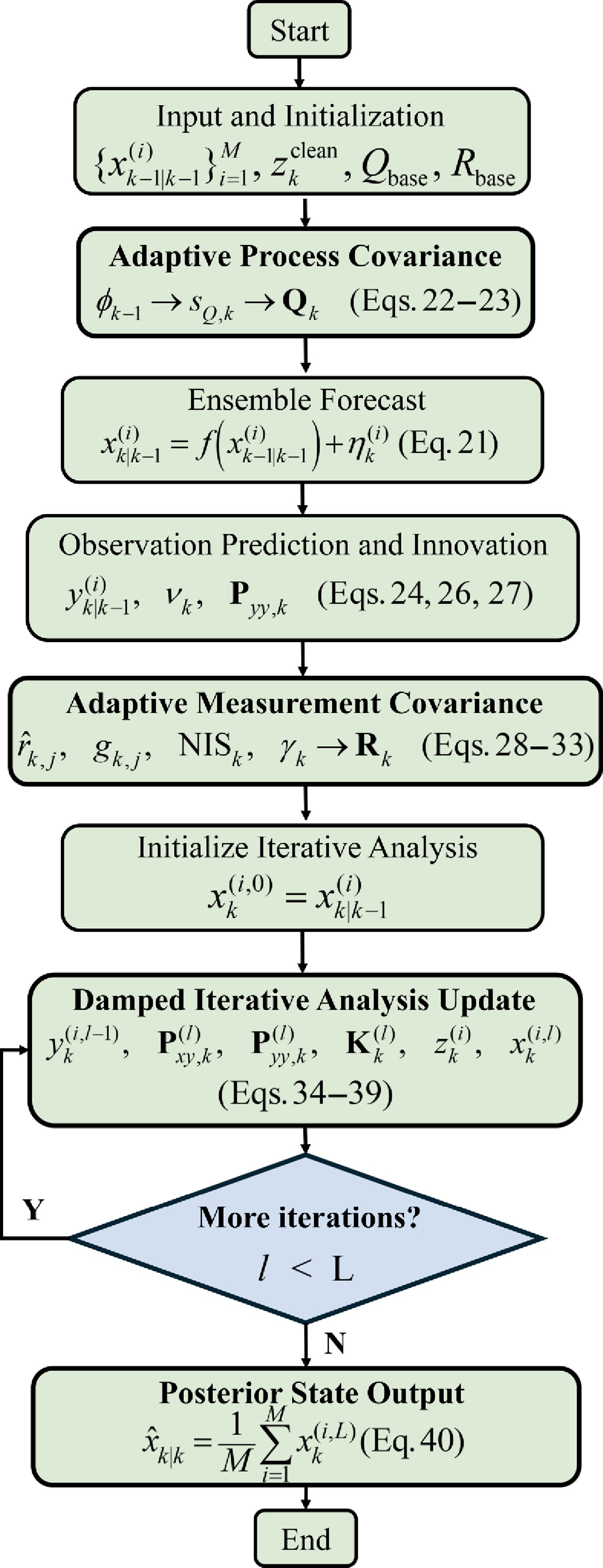
Figure 3. 

Workflow of the proposed improved iterative ensemble Kalman filter backend.

Algorithm 1 summarizes the main procedure of the proposed IEnKF for indoor UWB localization. Unless otherwise stated, the main fixed filter parameters were kept the same across all repeated experiments:

● ensemble size: $ M=100 $;

● number of inner iterations: $ L=3 $;

● base process covariance: $ {\boldsymbol{Q}}_{{\rm{base}}}={\rm{diag}}(0.01,0.01,0.01, 0.01, 0.01,0.01) $;

● base measurement covariance: $ {\boldsymbol{R}}_{{\rm{base}}}={\rm{diag}}(0.50,0.50,0.50, 0.50) $;

● damping-factor sequence: $ [0.72,0.50,0.32] $.

The selection and robustness of the main empirical parameters are further examined through the parameter sensitivity analysis.

Statistical analysis

Localization performance was evaluated using both time-aligned reference-point-based statistics and trajectory-level path-deviation analysis. Sixteen predefined reference points were distributed along the rectangular experimental trajectory. For the $ j $^th reference point, the corresponding sampling instant is denoted by $ t_j^{{\rm{ref}}} $. For each localization method, the estimated position with the timestamp closest to $ t_j^{{\rm{ref}}} $ is selected for error calculation. The same set of reference-point sampling instants is used for all compared methods to avoid method-dependent temporal alignment differences.

The extracted estimated position and the corresponding predefined reference position are denoted by $ \hat{{\boldsymbol{p}}}_{j}^{{\rm{ref}}}=[\hat{x}_{j},\,\hat{y}_{j}]^{T} $ and $ {\boldsymbol{p}}_{j}^{{\rm{ref}}}=[x_{j}^{{\rm{ref}}},\,y_{j}^{{\rm{ref}}}]^{T} $, respectively. The corresponding localization error is defined as:

The overall reference-point localization accuracy is then quantified by:

Furthermore, the cumulative distribution function of the 16 reference-point errors is used to compare the error distribution of different methods. A steeper cumulative curve indicates stronger error concentration within a smaller range. This evaluation should be interpreted as a discrete reference-point-based assessment that complements the trajectory-level comparison.

This section presents the experimental evaluation of the proposed indoor two-dimensional UWB localization framework. To establish a clear connection between the algorithm design and the achieved localization performance, the experiments include a ranging-level assessment of the multi-channel UWB outlier removal module, localization comparison with representative filtering methods, ablation analysis of the proposed components, controlled robustness analyses under anchor-channel removal and synthetic ranging disturbances, and parameter sensitivity analysis.

The indoor UWB experimental configuration is shown in Fig. 4 and summarized in Table 1. To evaluate the proposed localization method, an indoor UWB system consisting of four fixed anchors and one mobile tag was established using Nooploop LinkTrack UWB modules, with the mobile tag mounted on the UAV platform. The target position was estimated from tag-to-anchor ranging measurements. The anchors were deployed around the experimental area to form an approximately rectangular observation region, within which the UAV moved along a predefined rectangular path. Repeated trials were conducted under identical conditions to examine the stability and repeatability of the proposed method.

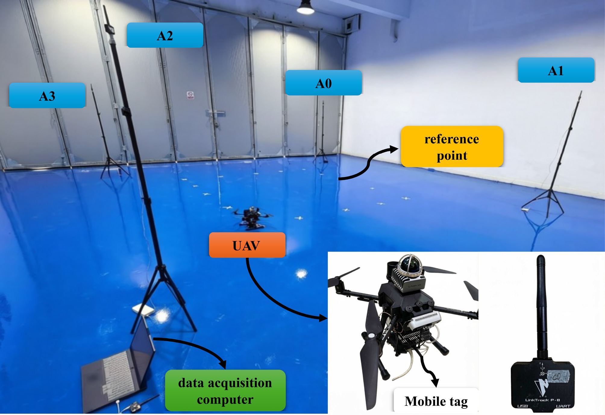
Figure 4. 

Experimental setup of the indoor UWB localization test, including four fixed anchors, the UAV-mounted mobile tag, reference points, and the data acquisition computer.

Since no external high-precision ground-truth system was available in the experiment, localization performance was evaluated using predefined reference points and the predefined rectangular path rather than a continuous absolute ground-truth trajectory. Specifically, 16 fixed reference points were defined along the predefined rectangular path. These points are sparse benchmark positions for repeatable quantitative comparison, not dense continuous ground truth. They are distributed along the four sides of the rectangular path and include both straight-line segments and corner regions, covering positions relatively close to anchors, positions farther from anchors, and turning regions where the motion state changes more noticeably. When the UAV passed the corresponding locations, the estimated position was compared with the associated reference point, and the resulting deviation was regarded as the positioning error at that point. Based on the errors at these 16 reference points, RMSE and MAE were computed as quantitative evaluation metrics. In addition, the two-dimensional estimated trajectories were compared with the predefined rectangular path to evaluate trajectory consistency. Therefore, the trajectory-level quantitative results reported below should be interpreted as path-deviation statistics rather than errors with respect to a dense external ground-truth trajectory.

The absence of an external high-precision ground-truth system also means that systematic biases may affect the interpretation of absolute localization accuracy. In the present UWB setup, possible systematic bias sources include anchor-coordinate surveying errors, fixed UWB ranging offsets, hardware calibration residuals, antenna installation offsets, reference-point marking errors, and nearest-sample time-alignment errors when the UAV passes predefined reference locations. These biases may introduce a common position shift, local deformation, or geometry-dependent error in the estimated trajectory. For example, anchor-coordinate errors and fixed range offsets can propagate through the range-based localization geometry and appear as position-domain biases. Therefore, the reported RMSE and MAE values should be interpreted as reference-point and path-deviation statistics under the same experimental configuration, rather than as a complete characterization of absolute positioning accuracy with respect to an external high-precision ground-truth trajectory. Since all compared methods use the same anchor coordinates, UWB measurements, reference points, and evaluation procedure, the comparative performance improvement remains meaningful, while the absolute error values may still contain common systematic-bias components.

Performance evaluation of multi-channel UWB outlier removal

To mitigate the adverse influence of abnormal ranging observations on subsequent localization, the proposed multi-channel UWB outlier removal method was first evaluated at the ranging level. This preprocessing procedure aims to identify and suppress spike noise, local abrupt changes, and short-duration abnormal fluctuations in the raw UWB measurements, thereby improving the consistency of the ranging inputs used for state estimation.

Figure 5 shows the front-end preprocessing result for one representative experimental run. In this figure, the raw UWB ranging sequences from the four anchor channels are compared with the corresponding preprocessed sequences, and the samples identified as abnormal ranges by the proposed multi-channel outlier removal module are highlighted in red. This visual comparison illustrates how spike-like disturbances and short-duration abnormal fluctuations are suppressed before the cleaned UWB measurements are supplied to the backend localization filter.

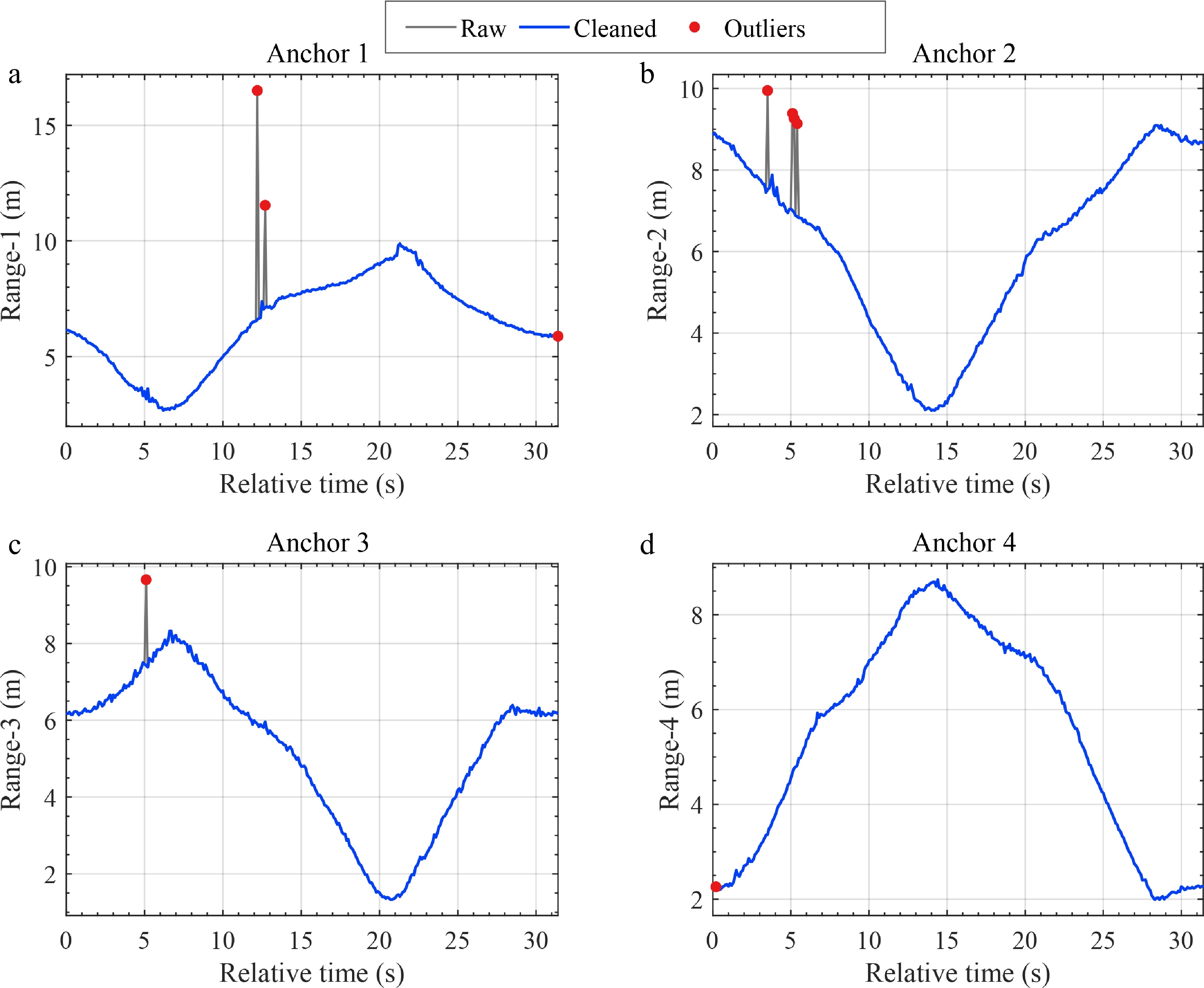
Figure 5. 

UWB range measurements before and after multi-channel outlier removal in one representative experimental run.

Since manually annotated outlier ground truth was not available in the experiment, the detection accuracy of the front-end module could not be directly computed. Instead, the preprocessing performance was quantitatively evaluated using the detected outlier count, detected outlier ratio, and the reduction of UWB ranging residual statistics before and after preprocessing. The results averaged over four experimental runs are shown in Table 2.

In Table 2, the ranging residual is computed with respect to the local median baseline generated by the sliding-window median operation in the front-end outlier removal module. For each UWB channel, it is defined as the difference between the ranging observation and the corresponding local median baseline, and the raw and preprocessed sequences are evaluated using the same residual definition. This local-median-based residual provides a channel-wise measure of short-term inconsistency around the local ranging trend, and is therefore used to quantify whether the front-end preprocessing suppresses abnormal local fluctuations. The results show that preprocessing reduces the ranging residual standard deviation for all four anchors, from $ 0.1708 $–$ 0.4718 $ m before preprocessing to $ 0.0594 $–$ 0.2308 $ m after preprocessing. The largest reductions are observed for Anchor 2 and Anchor 3, which also have relatively higher detected outlier ratios. These results indicate that local abnormal fluctuations are effectively suppressed and cleaner inputs are provided for subsequent state estimation.

Localization performance and robustness evaluation

Baseline localization performance

To evaluate the effectiveness of the proposed method in indoor two-dimensional UWB localization, comparative experiments were conducted using the same dataset and the same four-anchor ranging conditions. The compared methods include the extended Kalman filter (EKF), unscented Kalman filter (UKF), ensemble Kalman filter (EnKF), maximum correntropy criterion-based unscented Kalman filter (MCC-UKF), robust adaptive cubature Kalman filter (RA-CKF), and the proposed IEnKF. These methods were selected because they represent conventional, ensemble-based, robust, and adaptive filtering paradigms for nonlinear UWB state estimation, while MCC-UKF and RA-CKF were included as representative robust/adaptive baselines for non-Gaussian ranging errors, NLOS disturbance, and measurement outliers.

The EKF, UKF, EnKF, MCC-UKF, and RA-CKF methods were implemented as filtering baselines that directly use the raw UWB ranging measurements without the proposed front-end outlier removal module. In contrast, the proposed method first applies the multi-channel UWB outlier removal module and then performs localization using the improved iterative ensemble Kalman filter, thereby combining measurement preprocessing and robust recursive state estimation within a unified framework. Therefore, the following comparison mainly evaluates the overall performance of the proposed pipeline against conventional, robust, and adaptive filtering baselines under the same four-anchor UWB dataset. The original localization output provided by the Nooploop system is also included in the trajectory comparison in Fig. 6 as an auxiliary qualitative reference, but it is not used as a filtering baseline in the quantitative tables.

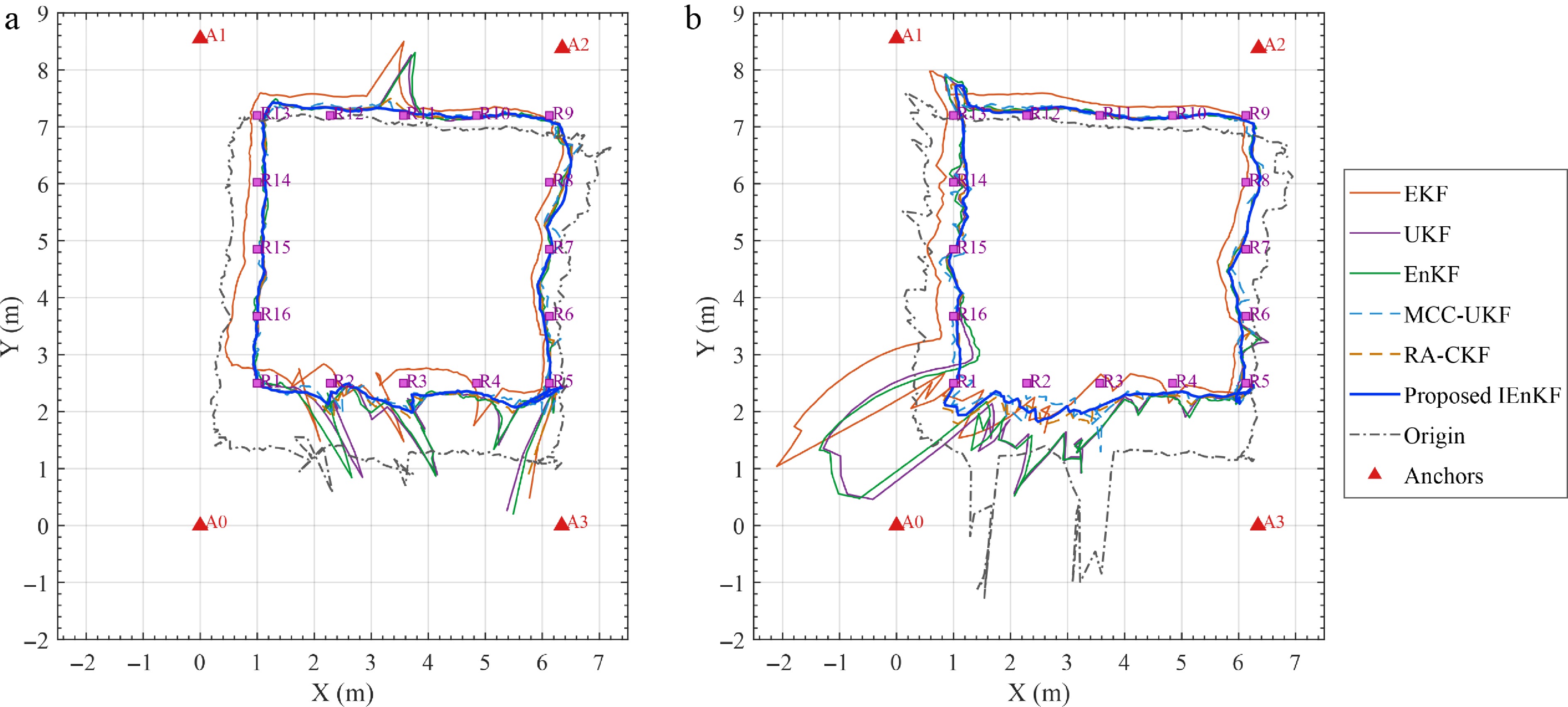
Figure 6. 

Two-dimensional trajectory comparison of different localization methods in two representative experimental runs. (a) Representative run 1. (b) Representative run 2.

Localization performance was evaluated from both qualitative and quantitative perspectives. The qualitative analysis focused on the consistency of the two-dimensional estimated trajectories, whereas the quantitative analysis was based on the positioning errors at the 16 predefined reference points and the corresponding RMSE and MAE values.

Figure 6 shows two representative experimental runs. In both runs, the proposed framework follows the predefined rectangular path more consistently than the original Nooploop output and the baseline filters.

Figure 7a shows representative path-deviation results, Fig. 7b shows reference-point positioning errors, and Table 3 summarizes the trajectory-level path-deviation accuracy and reference-point localization accuracy of the compared methods.

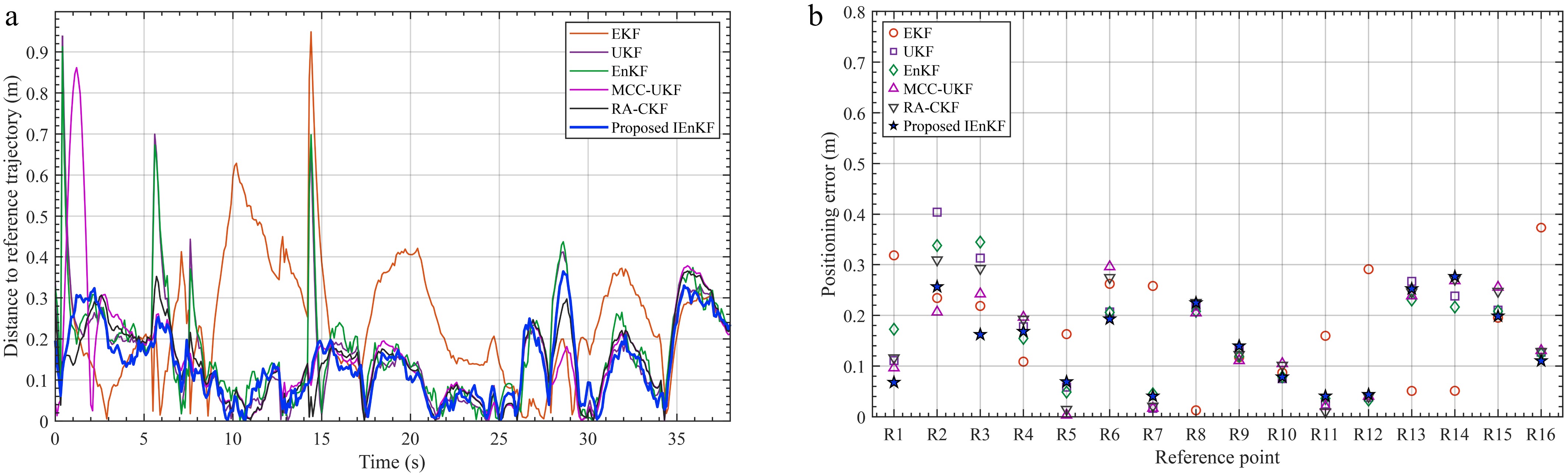
Figure 7. 

Trajectory-to-reference-path deviation and reference-point positioning error comparison of different filtering methods in one representative experimental run. (a) Trajectory-to-reference-path deviation. (b) Reference-point positioning error.

As shown in Table 3, the proposed IEnKF obtains the best path-deviation and reference-point metrics among the compared filtering methods, indicating improved trajectory consistency and reference-point localization accuracy under the same four-anchor UWB dataset. Figure 7b further shows smaller and more balanced reference-point errors for the proposed framework in the representative run.

Figure 8 further shows that the proposed framework concentrates more reference-point errors within a smaller range, supporting the reference-point accuracy trend in Table 3.

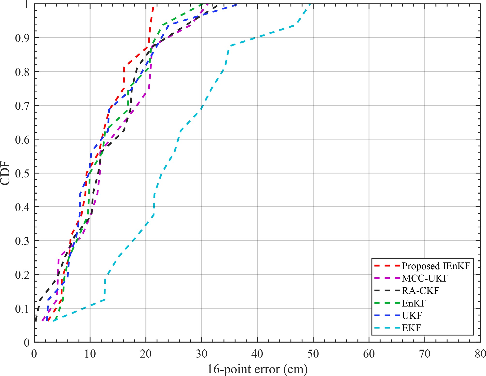
Figure 8. 

CDF curves of reference-point positioning errors for different filtering methods in one representative experimental run.

To further analyze the computational efficiency and embedded implementation feasibility of the proposed method, the algorithmic complexity of the IEnKF backend was examined. In the present two-dimensional UWB localization formulation, the state vector consists of horizontal position, velocity, and acceleration components, namely $ {\boldsymbol{x}}_k=[x_k,y_k,v_{x,k},v_{y,k},a_{x,k},a_{y,k}]^T $, so the state dimension is $ n=6 $. The measurement vector is composed of four anchor-to-tag UWB ranges, so the measurement dimension is $ m=4 $. The adopted IEnKF configuration uses an ensemble size of $ M=100 $ and a fixed inner iteration number of $ L=3 $. For one filtering update, the main computational cost comes from ensemble prediction, nonlinear UWB range-observation propagation, sample covariance calculation, channel-aware measurement covariance construction, and damped iterative ensemble analysis. The dominant computational complexity can be expressed as

Under the adopted setting of $ n=6 $, $ m=4 $, $ M=100 $, and $ L=3 $, the computational burden mainly scales linearly with the ensemble size and the number of inner iterations. Moreover, the matrix inversion in the Kalman-type update is only performed on a $ 4\times4 $ observation covariance matrix. Therefore, although the proposed IEnKF is computationally heavier than conventional EKF, UKF, EnKF, MCC-UKF, and RA-CKF baselines, its computation remains low-dimensional and lightweight. From an embedded implementation perspective, the proposed filtering backend is suitable for STM32H743-class microcontrollers with a 480 MHz ARM Cortex-M7 core. Since the UWB system used in this study operates at 10 Hz, corresponding to a 100 ms sampling interval, the computational scale of the proposed filter is compatible with the real-time requirement of the UWB localization system. In addition, the proposed method does not require GPU acceleration, image feature extraction, or neural-network inference, which makes it suitable for resource-constrained indoor UAV platforms.

Method-component analysis

To further examine whether the observed performance gain is solely associated with front-end outlier removal, an additional comparison among backend filters was conducted under the same cleaned UWB measurements. In this experiment, EKF, UKF, EnKF, and the proposed method all used the same preprocessed ranging data as input, so that the influence of measurement quality was controlled and the comparison mainly reflected the difference in backend filtering capability.

As shown in Table 4, under the same cleaned measurement input, the proposed method still achieves the lowest RMSE and MAE among all compared methods. This suggests that the performance improvement of the proposed framework is associated not only with the improvement in front-end observation quality but also with the robustness of the backend filtering strategy.

Figure 9 shows that, under the same cleaned measurements, the proposed backend still provides better trajectory consistency and smaller reference-point errors.

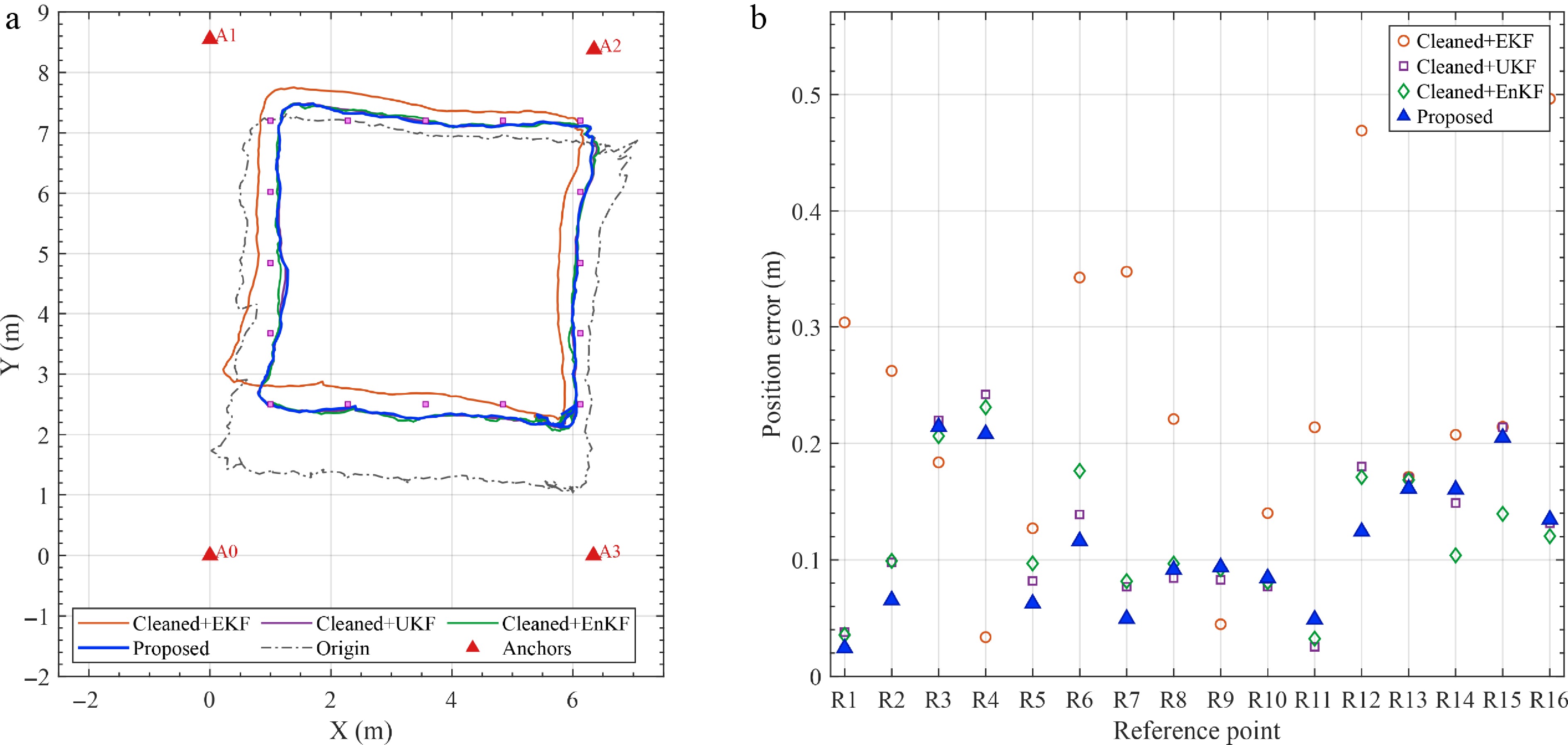
Figure 9. 

Backend filter comparison under the same cleaned UWB measurements in one representative experimental run. (a) Two-dimensional trajectory comparison. (b) Reference-point positioning errors.

Although the above comparisons demonstrate the overall advantage of the proposed framework over the baseline methods, they do not explicitly distinguish the respective contributions of the front-end multi-channel UWB outlier removal and the back-end improved iterative ensemble Kalman filtering. To further clarify their roles in the final performance, an ablation study was conducted.

Specifically, four configurations were considered: Raw + EnKF, Cleaned + EnKF, Raw + IEnKF, and Cleaned + IEnKF. Here, 'Raw' and 'Cleaned' indicate whether the ranging data were directly used or first preprocessed by the proposed multi-channel UWB outlier removal module, while 'EnKF' and 'IEnKF' denote the standard ensemble Kalman filtering backend and the improved iterative ensemble Kalman filtering backend, respectively.

Table 5 shows that both front-end preprocessing and the improved iterative backend contribute to the final performance. Cleaned + IEnKF achieves the best result, indicating complementary benefits from measurement refinement and robust recursive filtering.

A component-level ablation study was further conducted using the same cleaned UWB measurements.

The baseline EnKF uses none of the three proposed backend mechanisms.

The remaining variants remove adaptive $ {\boldsymbol{Q}} $, channel-aware $ {\boldsymbol{R}} $, or damping one at a time.

As shown in Table 6, the full proposed backend achieves the best overall performance, with the lowest RMSE, MAE, and maximum error. Removing the channel-aware measurement covariance causes the largest degradation, increasing the RMSE from 0.1451 to 0.1682 m and the maximum error from 0.2820 to 0.3792 m. This indicates that accurately representing channel-dependent UWB measurement uncertainty is the most influential backend component in the tested indoor environment. Removing the adaptive process covariance or the damping strategy also degrades the results, although their effects are smaller. These results show that all three backend mechanisms contribute to the final performance, while the channel-aware measurement covariance plays the dominant role in improving robustness against nonuniform ranging disturbances.

Figure 10 illustrates the same trend in a representative run: Cleaned + IEnKF stays closest to the expected path and has the most favorable error distribution. Overall, the ablation results show that front-end outlier removal and backend iterative filtering provide complementary improvements.

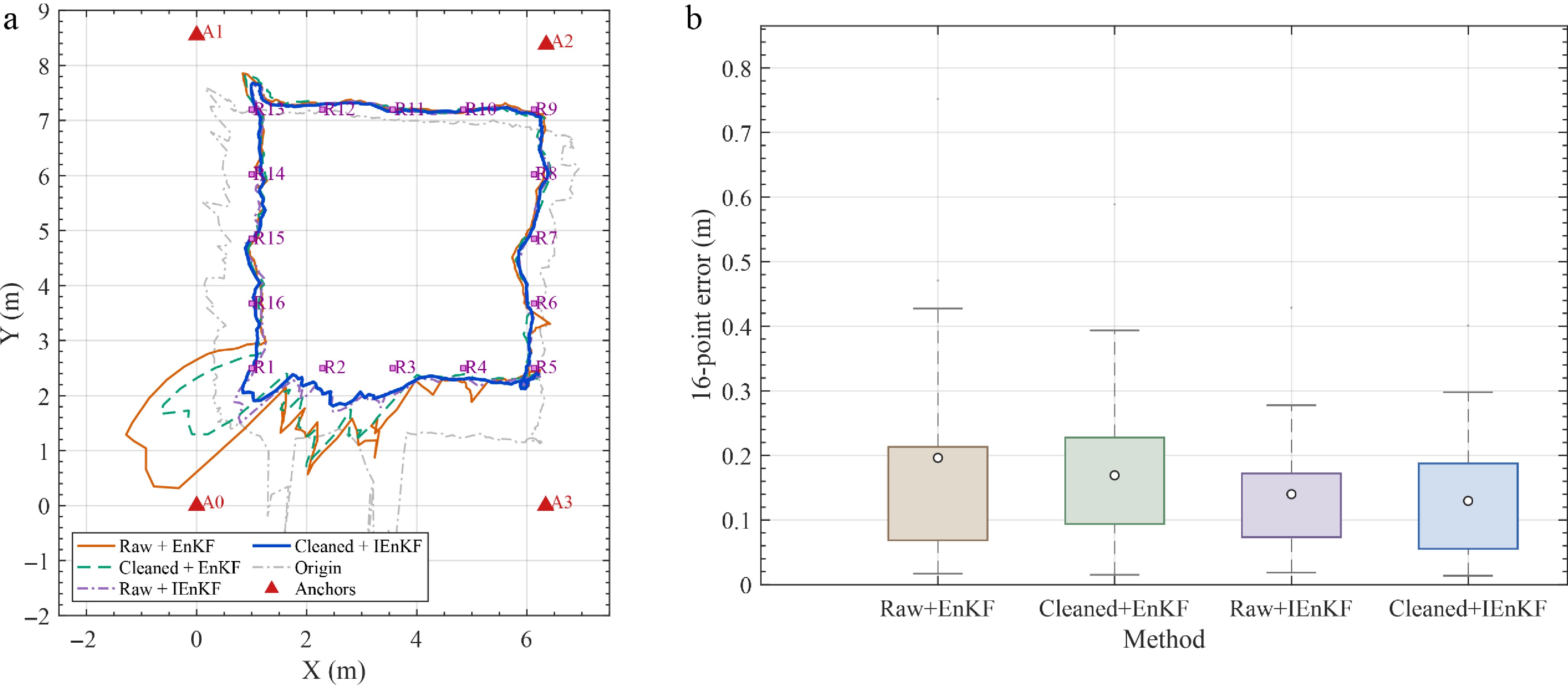
Figure 10. 

Ablation comparison of different front-end and back-end configurations in one representative experimental run. (a) Two-dimensional trajectory comparison. (b) Reference-point positioning error distribution.

Robustness analysis

To further examine the robustness of the proposed framework beyond the original four-anchor evaluation, additional controlled analyses were conducted based on the existing four repeated UWB experimental runs. These analyses were performed in post-processing rather than through newly collected physical LOS/NLOS flight trials. Specifically, anchor-configuration robustness was evaluated by selectively removing one anchor channel from the recorded four-anchor measurements, and disturbed-ranging robustness was evaluated by injecting synthetic NLOS-like positive ranging biases and dynamic-occlusion-like burst disturbances into the recorded UWB ranging sequences. Therefore, the added results should be interpreted as controlled data-level stress tests for robustness evaluation, not as newly collected real NLOS or physical occlusion experiments.

First, the influence of anchor availability and anchor geometry was evaluated by selectively removing one anchor channel from the recorded four-anchor measurements during post-processing. This analysis emulates anchor-channel removal or degraded anchor availability while keeping the original trajectory and recorded measurements unchanged. Second, to examine robustness against NLOS-like and occlusion-like ranging degradation, synthetic disturbances were introduced into the recorded UWB ranging sequences. The synthetic NLOS cases were generated by adding positive ranging biases to randomly selected measurements with different disturbance ratios, while the dynamic occlusion case was generated by introducing burst-type disturbance segments. The same perturbed ranging sequences were used for all compared methods to ensure a fair comparison. The results of these controlled robustness analyses are summarized in Table 7.

As shown in Table 7, the original four-anchor configuration achieves the best overall accuracy, with an RMSE of 0.1451 m and an MAE of 0.1243 m. After one anchor channel is removed, the localization performance varies with the retained anchor geometry. The A1-A2-A3 and A0-A1-A2 configurations still maintain relatively small RMSE values of 0.1679 and 0.1594 m, respectively, whereas the A0-A2-A3 and A0-A1-A3 configurations show larger errors. The proposed method can still provide valid estimates under all tested three-anchor configurations, although the accuracy clearly depends on the retained anchor geometry. In the synthetic disturbance tests, the proposed IEnKF achieves the lowest RMSE under all tested stress cases. Under 5%, 10%, and 15% synthetic NLOS bias conditions, its RMSE remains within 0.1575–0.1687 m, and it obtains the lowest RMSE of 0.1620 m under the dynamic occlusion stress test. These results provide supplementary evidence that the combination of front-end outlier suppression and backend adaptive iterative filtering improves robustness against synthetic NLOS-like positive bias and dynamic-occlusion-like burst disturbance.

Parameter sensitivity analysis

A compact parameter sensitivity analysis was conducted to examine whether the performance improvement depends on a single carefully tuned parameter setting. During each test, only one parameter was varied while the remaining parameters were fixed at their recommended values. The tested front-end parameters include the Tukey cutoff values $ 2.5/3.0/3.5/4.0 $ and window sizes $ 5/7/9/11 $, and the tested backend parameters include ensemble sizes $ 30/50/80/100/120 $, iteration numbers $ 1/2/3/4/5 $, $ {\boldsymbol{Q}} $ scaling bounds $ 2/3/4/5 $, and $ {\boldsymbol{R}} $ clipping bounds $ 1.5/2.5/3.5/4.5 $.

As shown in Table 8, the recommended values are Tukey cutoff $ 2.5 $, window size $ 7 $, ensemble size $ 100 $, iteration number $ 3 $, $ {\boldsymbol{Q}} $ scaling bound $ 2 $, and $ {\boldsymbol{R}} $ clipping bound $ 1.5 $. The 'Avg. best RMSE' values in this table are obtained from one-factor sensitivity sweeps and may therefore be slightly lower than the main comparison result under the fixed reported configuration; they are used to characterize local parameter sensitivity rather than to redefine the baseline performance reported in Table 3. The corresponding RMSE variation ranges are $ 0.0022 $, $ 0.0030 $, $ 0.0098 $, $ 0.0201 $, $ 0.0000 $, and $ 0.0118 $ m, respectively. The Tukey cutoff, window size, ensemble size, $ {\boldsymbol{Q}} $ scaling bound, and $ {\boldsymbol{R}} $ clipping bound exhibit low sensitivity, whereas the iteration number shows medium sensitivity. These results indicate that the reported improvement is not caused by a single carefully tuned parameter setting. In practical use, the recommended parameters provide a balanced configuration between localization accuracy, robustness, and computational cost.

The present study shows that indoor UWB localization performance can be improved by jointly addressing measurement reliability and recursive estimation robustness. These two aspects are closely coupled because corrupted ranging observations caused by multipath propagation, transient occlusion, NLOS propagation, and channel inconsistency can directly degrade subsequent state estimation^[8,9]. By combining multi-channel outlier removal with adaptive iterative ensemble filtering, the proposed framework improves both the quality of the observations entering the filter and the robustness of the recursive update. Under the same indoor UWB conditions, it achieves better trajectory consistency and reference-point positioning accuracy than the comparison methods. The lower RMSE and MAE indicate more accurate and stable localization at representative evaluation locations, while the cumulative error distribution shows that more positioning errors are concentrated within a smaller range. These findings support a joint front-end observation-quality and backend filter-robustness design for disturbance-prone indoor UAV applications. They are also consistent with recent robust UWB filtering studies, in which maximum-correntropy-based UKF and robust adaptive CKF strategies were introduced to reduce the influence of non-Gaussian ranging errors, NLOS effects, model mismatch, and measurement outliers^[26,27]. Compared with these backend-oriented methods, the proposed framework further emphasizes the joint design of front-end channel-wise range correction and backend adaptive iterative ensemble filtering.

The Gaussian-noise formulation in the state-space model is used as a nominal covariance-based approximation for recursive filtering, not as a strict statistical assumption for raw UWB ranging errors. The front-end Tukey module suppresses or reconstructs severe abnormal measurements, after which the residual errors may be more compatible with a covariance-based update but are still not assumed to be perfectly Gaussian. Similar covariance-based robust and adaptive ensemble filtering ideas have been used to improve nonlinear filtering performance under model error, sampling uncertainty, and non-Gaussian observation disturbances^[22−25]. In the present implementation, residual non-Gaussian effects, channel-dependent uncertainty, and motion-model mismatch are handled through adaptive $ {\boldsymbol{Q}}_k $, channel-aware $ {\boldsymbol{R}}_k $, covariance clipping, small regularization terms, fixed small iteration numbers, and damped iterative updates. These mechanisms improve practical robustness and numerical stability by limiting unrestricted covariance growth and excessive nonlinear correction, while leaving formal global stability and asymptotic convergence analysis as an open theoretical issue.

The two-dimensional formulation defines the practical scope of the present work. The study focuses on horizontal localization because reliable pure-UWB height estimation remains challenging in many indoor deployments, especially when anchors are mounted at similar heights or near surrounding walls. Such geometry can produce weak vertical observability and make altitude estimates more sensitive to ranging noise, NLOS propagation, and multipath disturbance than horizontal estimates. The experiments were therefore conducted along a predefined planar path, with available reference positions defined on the ground plane. This setting does not demonstrate full three-dimensional flight, such as takeoff, landing, altitude changes, obstacle-avoidance maneuvers, or aggressive vertical motion. Nevertheless, two-dimensional UWB localization remains relevant for fixed-height indoor inspection, warehouse aisle patrol, inventory scanning, horizontal-layer mapping, and station-keeping at known working heights, where altitude stabilization can be handled by barometers, laser rangefinders, visual odometry, lidar, or IMU-assisted height estimation.

Extending the present formulation to three-dimensional localization is conceptually feasible but requires several engineering changes. The state-space model should include vertical position, velocity, and acceleration components so that the filter can estimate the $ x $-, $ y $-, and $ z $-direction motions jointly, and the UWB observation model should be extended from the current planar range equation to a 3D Euclidean range equation that includes both anchor height and UAV altitude. Reliable 3D UWB localization also requires suitable anchor deployment and sufficient vertical observability, with non-coplanar anchors and adequate height diversity. If the anchors are nearly coplanar, the vertical component may remain weakly observable, and the altitude error may be amplified even when the horizontal position can be estimated reasonably well. Additional anchors may also be required to improve geometric dilution, maintain redundancy under NLOS blockage, and stabilize adaptive covariance estimation. This requirement is consistent with recent UWB sensor-placement studies, which show that both radio geometry and obstacle-induced NLOS bias affect localization quality, and that optimized UWB radio placement can substantially improve localization accuracy in both 2D and 3D settings^[28].

The evaluation protocol also affects the interpretation of the quantitative results. Because no external high-precision reference system was available, the predefined reference points and rectangular path provide a repeatable basis for comparative reference-point and path-deviation evaluation, rather than dense external ground truth. The reported errors may include systematic components from anchor-coordinate surveying errors, fixed ranging offsets, hardware installation offsets, reference-point marking uncertainty, and nearest-sample time-alignment errors. The proposed framework can reduce abnormal ranging fluctuations, channel-dependent disturbances, and time-varying inconsistencies, but it does not calibrate all absolute systematic biases in the experimental setup. This reading is consistent with previous UWB localization studies showing that commercially available UWB radios may suffer from measurement bias and outliers, and that bias correction or robust filtering is often required for reliable deployment on resource-constrained mobile robots^[29].

The added anchor-channel removal and synthetic ranging-disturbance analyses broaden the evaluation as controlled post-processing stress tests based on the existing dataset. They provide repeatable degraded-ranging comparisons, but they are not newly collected physical LOS/NLOS or dynamic-occlusion experiments. The main limitations are therefore the planar UWB-only formulation, the absence of external high-precision ground truth, the use of a rectangular trajectory and predefined reference points, and validation in one indoor environment with a fixed four-anchor deployment. Further development should include cross-environment validation under different indoor layouts, more diverse trajectory types, high-precision motion-capture or other external reference systems, multi-height and non-coplanar anchor deployment optimization, full 3D localization with UWB/IMU fusion^[30], integration of complementary altitude-related sensors, and physical LOS/NLOS and dynamic-occlusion tests under different disturbance conditions.

This paper proposes a robust indoor UAV UWB localization framework that combines multi-channel UWB outlier removal with an improved iterative ensemble Kalman filter. By integrating local-Tukey-reweighting-based preprocessing with adaptive and iterative ensemble filtering, the proposed method improves both measurement reliability and estimation robustness under unreliable indoor UWB ranging conditions and controlled synthetic disturbance tests. Experimental results in a four-anchor indoor UWB setup demonstrate that the proposed framework outperforms EKF, UKF, standard EnKF, MCC-UKF, and RA-CKF in terms of trajectory consistency, reference-point positioning accuracy, and the RMSE and MAE computed from predefined reference-point errors. Overall, the proposed framework provides a practical solution for two-dimensional UAV localization in GNSS-denied indoor environments with unreliable ranging conditions. Future work should examine broader validation, full 3D extension with non-coplanar anchors, physical LOS/NLOS or occlusion conditions, and high-precision external reference systems.