Intent-informed UAV tracking for evasive targets in urban environments

Unmanned aerial vehicles (UAVs)^[1] are now widely deployed across diverse applications, such as communication services^[2], reconnaissance and surveillance^[3,4], search and rescue^[5,6], ground mapping^[7], and agriculture^[8,9]. Among them, for military and civilian applications, searching for and tracking targets in a given region has great demand and has been heavily researched^[10,11]. In addition, with accelerated urbanization around the world, UAVs are increasingly being used for various tasks in urban environments. The use of UAVs for searching for and tracking targets in urban environments has received continuous attention^[12,13].

Conventional target tracking typically follows a predict-then-plan paradigm: The target's future motion is first estimated, and the UAV's actions are then chosen to increase the future detection likelihood or reduce state uncertainty. This paradigm is instantiated across recent work. Yu et al.^[14] proposed a path planner for tracking a moving target in urban contexts using a dynamic occupancy grid and Bayesian filtering, coupled with a tree-search strategy that maximizes the cumulative detection probability over a finite horizon. Cook et al.^[15] improved ground-target observation in urban settings by learning a data-driven motion model from observed behaviors and fusing it with a traditional model to refine trajectory prediction. Yao et al.^[16] cast tracking as a model predictive control (MPC) problem and solved it with an enhanced grey wolf optimizer to obtain multi-UAV trajectories, while predicting target motion via an unscented Kalman filter. Qi et al.^[17] assumed multiple motion models and applied an interacting multiple model (IMM) filter with state–vector fusion for prediction. Hu et al.^[18] framed the search for and tracking of an unknown ground target as a fuzzy multiobjective path planning problem within a distributed predictive control framework, using an extended Kalman filter (EKF) for road-constrained motion and probability estimates near intersections. Collectively, these studies exemplify the predict-then-plan approach, differing in their predictive models and planning schemes yet sharing reliance on model-based state estimation to guide the choice of action.

Learning-based methods have also been explored for target tracking^[19,20]. Bhagat et al.^[21] developed a deep reinforcement learning (DRL) controller based on deep Q-networks (DQN) for urban target tracking. To improve generalization under uncertain target motion, Li et al.^[22] introduced Meta-TD3, which couples meta-learning with twin delayed deep deterministic policy gradient (TD3). Li et al.^[23] proposed an online path planner grounded in the deep deterministic policy gradient (DDPG) to handle maneuvering targets and obstacle avoidance. For multi-UAV tracking in dynamic environments where direct target information is limited, Jiao et al.^[24] proposed a multiagent reinforcement learning algorithm named MAA2CE. By integrating prioritized experience replay and network evolution mechanisms, this approach effectively addresses the multitarget tracking problem for UAV swarms operating in dynamic environments.

Despite extensive progress, comparatively few studies have focused on targets that actively evade tracking. Evasive maneuvers in complex environments pose a critical challenge because of their diversity and adaptability, manifested through high-speed maneuvering^[25], dynamic trajectory uncertainty^[26], occlusion avoidance^[27], and multitarget cooperative evasion^[28], with some targets using adversarial strategies^[29,30]. Quintero et al.^[31] formulated a method of UAV tracking of an evasive ground vehicle using a model of predictive control with moving horizon estimation, where the target's policy maximizes separation from UAVs. In a related game-theoretic setting^[32], the target maximizes distance while UAVs minimize it, and the UAVs infer the target's intelligence levels from observations to adapt their policies. Zhang et al.^[33] developed a closed-loop control strategy based on a minimax search tree with pruning informed by structural properties of the Kalman filter (KF), planning nongreedy control sequences to minimize worst-case target estimation uncertainty. Mbam et al.^[26] proposed a three-dimensional optimal tracking algorithm with a two-step predictive control strategy to follow ground targets that execute sharp evasive turns. When the target's speed exceeds the UAV's flight speed, a double-delayed deep deterministic policy gradient method has been used for multi-UAV cooperative pursuit of high-speed targets^[25]. Within a pursuit–evasion framework where the target uses artificial potential fields for escape, Chen et al.^[29] developed an encirclement strategy that integrates DRL with trajectory prediction to enable multi-UAV pursuit and encirclement in cluttered environments.

Even with these advances, maintaining continuous tracking of highly evasive targets remains difficult. Once contact is lost, reacquisition is costly and uncertain, as goal-directed adversarial maneuvers undermine reactive, kinematics-only trackers. This motivates intent reasoning: By inferring high-level goals and constraints, forecasting strategic trajectories, and quantifying uncertainty over intentions, a tracker can plan anticipatory information-seeking motions that preserve contact, resist deception, and improve continuity and robustness in contested environments.

Intent inference has been actively studied in autonomous driving^[34,35] and human–robot interaction^[36]. Karasev et al.^[37] modeled pedestrian intention as a policy within a Markov decision process under approximately rational behavior, using a Rao–Blackwellized filter to forecast long-term motion. In another line of work^[38], vehicle intention is represented by discrete high-level behaviors together with future trajectories, and an end-to-end learnable neural network jointly predicts both. Human behavior and intention have also been captured via an intention-driven dynamics model that encodes intention-dependent dynamics in latent states from noisy, high-dimensional observations^[39]. Similarly, Jain et al.^[40] defined intention as the agent's intended goal and behavior as goal-directed actions with varying rationality, and used recursive Bayesian filtering over multiple nonverbal cues to infer human intentions.

Building on these insights, this paper addresses the continuous tracking of a moving ground target exhibiting evasive behavior in urban environments using a single UAV. Evasive maneuvers can cause persistent loss of contact, especially under occlusions and limited sensing. To mitigate the constraints of limited UAV resources, we deploy ground sensors^[41,42] throughout the urban area to augment situational awareness and assist reacquisition when the target is lost. We model the target's intention as its goal region and infer candidate goal regions from the observed trajectories; these inferred intentions then condition the prediction of the target's future motion. Finally, we plan the UAV's actions to maximize the cumulative future detection probability, thereby improving tracking continuity against evasive targets in urban settings.

The main contributions of this work are as follows.

(i) Continuous tracking of evasive targets is enabled through explicit intent inference. When contact is lost, plausible escape trajectories are generated by sampling inferred goal-region intentions, providing principled guidance for anticipatory UAV planning and allowing rapid reacquisition and tracking resumption.

(ii) A method is proposed for real-time estimation and update of the target's behavior parameters from streaming trajectory observations when these parameters are initially unknown. In simulation, real-time parameter updates are shown to significantly enhance tracking continuity and overall UAV performance.

This study addresses the problem of using a UAV $ U $ to track an evasive target $ T $ in an urban setting $ \Omega $, as illustrated in Fig. 1. For tractability, the urban environment is abstracted as a directed graph $ M=(V,E) $ and a set $ C $. The directed graph $ M=(V,E) $ represents the layout of the roads of the urban environment, where each road is represented by an edge $ e(e\in E) $ and each road intersection is represented by a node $ v(v\in V) $. The set $ C $ consists of the ground sensors installed at road intersections, where each ground sensor $ c(c\in C) $ can sense the state of the target when it enters the sensor's sensing field $ {S}_{c} $ and sends the target information to the UAV. We use a circular area of radius $ R_{S}^{c} $ to represent the sensor's sensing field $ {S}_{c} $.

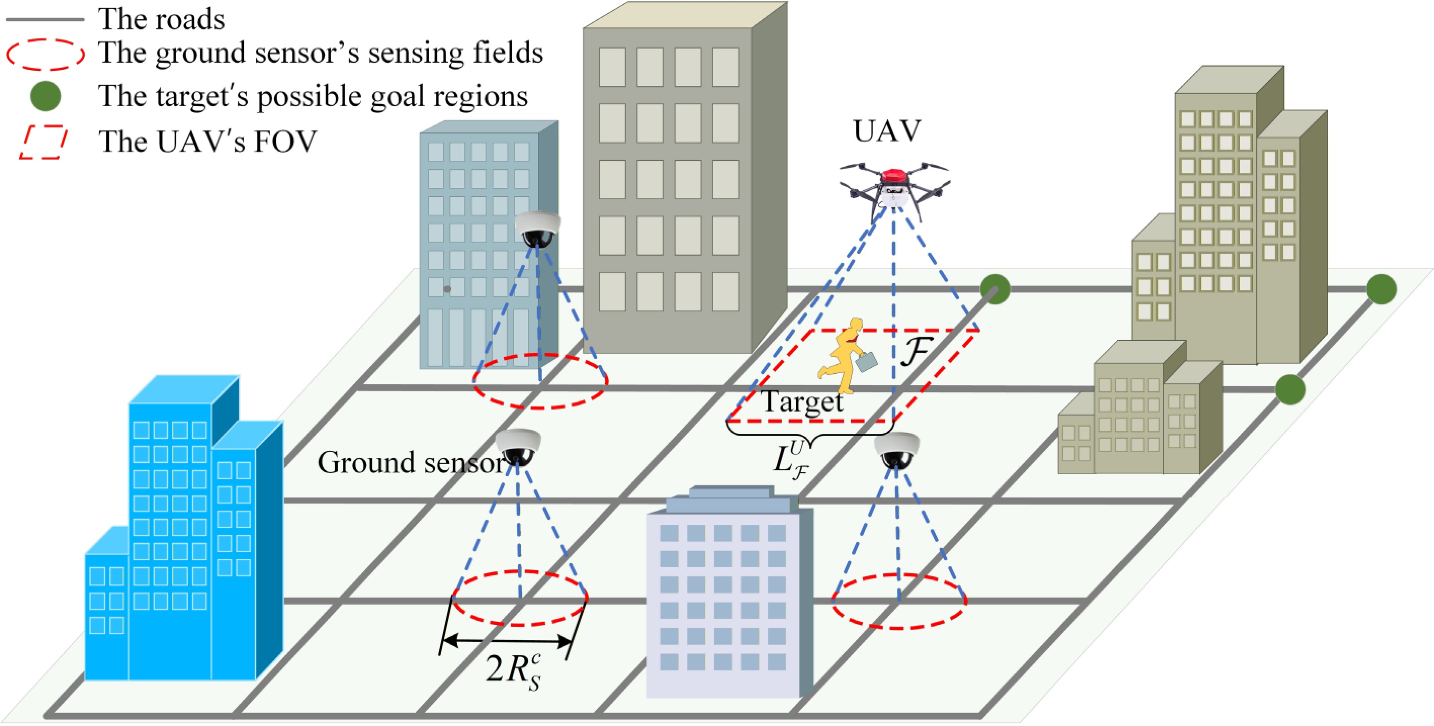
Figure 1. 

Schematic diagram of the problem scenario.

The target is assumed to possess a high-level intention of reaching a specific goal region $ {g}_{T} $, where $ {g}_{T}\in \mathbf{g} $ and $ \mathbf{g} $ denotes the set of all possible goal regions. The true goal region $ {g}_{T} $ is known only to the target itself. The target uses evasive maneuvers and may move beyond the UAV's field of view (FOV) $ \mathcal{F} $, resulting in loss of visual contact. The FOV $ \mathcal{F} $ is represented as a square with a side length $ L_{\mathcal{F}}^{U} $.

Let $ x_{T}^{t} $ and $ x_{U}^{t} $ denote the locations of the target and the UAV, respectively. Additionally, $ P(x_{T}^{t}) $ and $ P(x_{U}^{t}) $ represent the probabilities of the target being at $ x_{T}^{t} $ and the UAV being at $ x_{U}^{t} $, respectively. Let $ {D}_{t} $ denote the detection event, and let $ P({D}_{t}|x_{T}^{t},x_{U}^{t}) $ be the probability of detection when the UAV is at location $ x_{U}^{t} $ and the target is at location $ x_{T}^{t} $. The target detection probability $ P({D}_{t}|x_{T}^{t},x_{U}^{t}) $ is calculated as

where $ {\mathcal{F}}_{t} $ represents the UAV's FOV at time $ t $.

The UAV aims to maintain persistent tracking of the target as it moves toward its goal region. This objective is posed as an optimization problem as follows:

where $ {\pi }_{U} $ is the UAV's policy space.

We achieve continuous tracking through a closed-loop pipeline: (i) Update the posterior over the target's intentions from the latest observations; (ii) sample future target trajectories conditioned on this posterior; and (iii) plan the UAV's actions via a Monte Carlo tree search (MCTS)^[43] to maximize the expected cumulative detection under the generative model. After executing the chosen action, new observations update the posterior and the search tree is incrementally reused and extended. This belief–space coupling provides feedback without requiring an intractable joint optimization, and is essential for robustness under multimodal, evasive behavior. The system's framework is illustrated in Fig. 2.

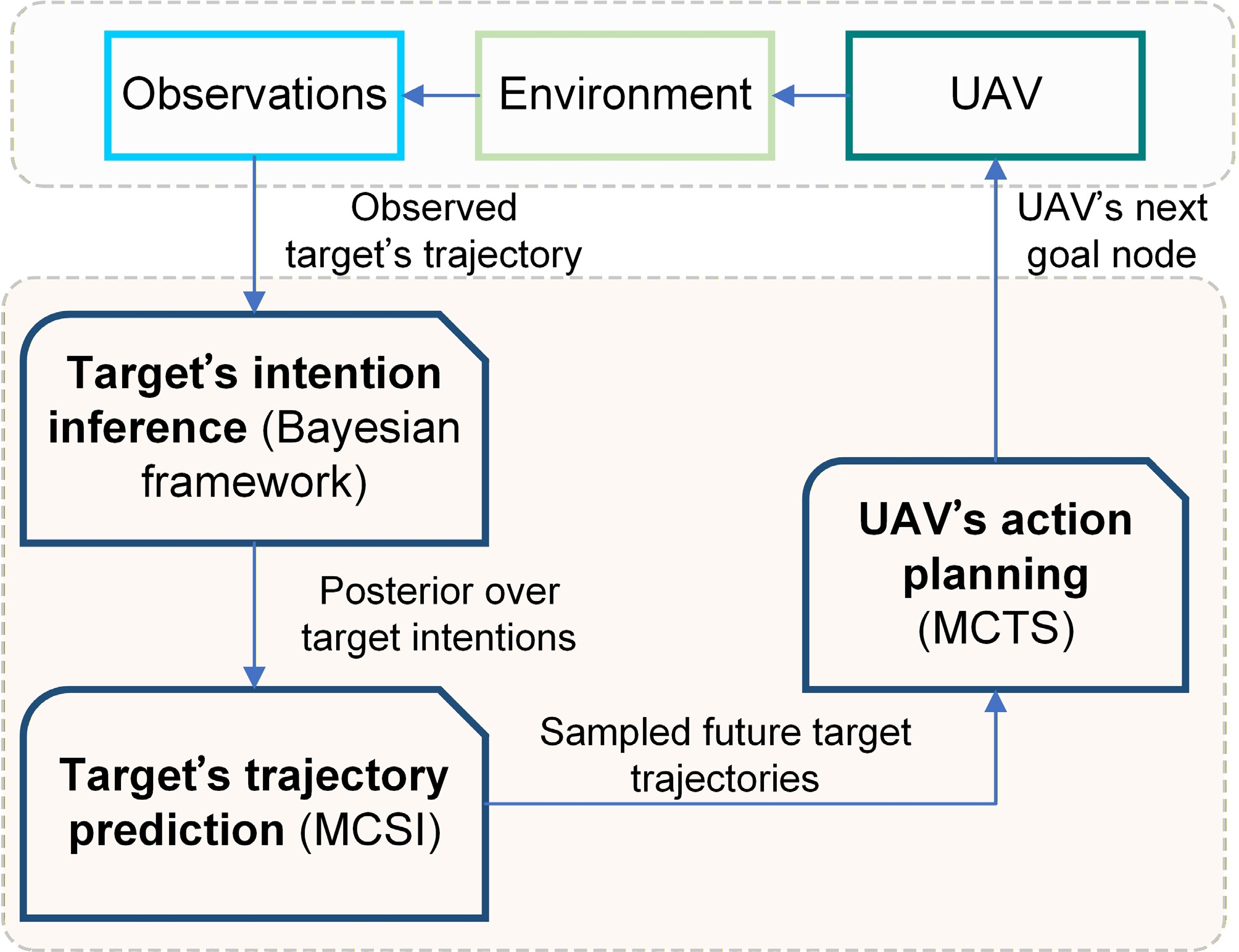
Figure 2. 

System framework.

Target's intention inference

A Bayesian scheme is used to sequentially estimate the target's intention. With $ x_{T}^{0:t} $ denoting the trajectory up to time t, the intention is updated as follows:

Under the inference scheme in (3), the target's intention is updated sequentially at each time step. To simplify the intention inference process, the target intention is updated only once when the movement of the target from node $ v_{T}^{c} $ to node $ v_{T}^{n} $ is observed by the UAV or ground sensors:

where $ P(v_{T}^{n}|v_{T}^{c},{g}_{T},\Omega ) $ is determined by the following equation:

where $ v_{T}^{c} $ and $ v_{T}^{n} $ represent the current and next road intersections, respectively;$ \rho (v_{T}^{c},v_{T}^{n},{g}_{T}) $ represents the distance from node $ v_{T}^{c} $, through node $ v_{T}^{n} $, to goal region $ {g}_{T} $; and$ \rho (v_{T}^{c},{g}_{T}) $ represents the distance from node $ v_{T}^{c} $ to the goal region $ {g}_{T} $. The normalization coefficient $ \eta $ is accordingly calculated by the following equation:

where $ \chi (v_{T}^{c}) $ represents the set of neighboring nodes of node $ v_{T}^{c} $.

The intention posterior is updated only when an observed transition between adjacent road network nodes provides new information regarding the target's route choice. If the target remains stationary or moves within the same road segment, the posterior over candidate goal regions is retained because no new intersection-level directional decision has been observed.

According to Equation (5), we assume that the target behaves as a rational agent, i.e., it always selects the shortest path to the goal region with the highest probability. Moreover, Equation (5) embodies the assumptions of goal-directed rationality and stochastic decision-making, while its role as a likelihood function ensures consistency with Bayesian inference. This integration enables the framework to robustly infer evasive targets' intentions by balancing prior knowledge with real-time behavioral observations.

When inferring the intention of the target through Equation (4), the behavior parameter $ \beta $ of the target is unknown and needs to be estimated. We estimate $ \beta $ in real time based on the observed target trajectory $ {\tau }_{t} $:

where $ {v}_{n-1} $, $ {v}_{n-2} $, and $ {v}_{n} $ represent the three nodes sequentially traversed by the target in the trajectory $ {\tau }_{t} $; $ {\hat{\beta }}_{n} $ is the estimated value of $ \beta $; and $ \delta \beta $ is the update step.

Target's trajectory prediction

Building on the inferred intentions, we introduce a trajectory prediction method that uses a Monte Carlo sampling technique to estimate the target's future trajectory. We name this method the Monte Carlo sampling technique with target intention (MCSI). In the MCSI approach, we sample $ N_{T}^{MC} $ trajectories that originate from the local goal node $ v_{T}^{l} $ and aim toward the goal region $ {g}_{i} $ ($ {g}_{i}\in \mathbf{g} $). The node $ v_{T}^{l} $ represents the local goal node observed prior to the target being lost. The sampling procedure allocates $ N_{i}^{MC} $ trajectories to the goal regions $ {g}_{i} $ according to their posterior probability as follows:

Each trajectory sample assumes the target moves at the speed measured at its latest observation. The local goal node of the target is selected using the probability calculated in (5) with the estimated target behavior parameter $ {\hat{\beta }}_{n} $, and the times $ {t}_{T}({v}_{i}) $ and $ {t}_{T}({v}_{j}) $ at which the target passes through the two adjacent nodes $ {v}_{i} $ and $ {v}_{j}({v}_{j}\in \chi ({v}_{i})) $ are recorded. By counting the time of passing two neighboring nodes in all sampled trajectories, the probability of finding the target between two neighboring nodes in a future time period $ [{t}_{1},{t}_{2}] $ can be obtained.

If the target transitions from $ {v}_{i} $ to $ {v}_{j} $, the UAV will similarly move from $ {v}_{i} $ toward $ {v}_{j} $. The probability of locating the target within the interval between these two neighboring nodes during the time period $ [{t}_{1},{t}_{2}] $ can be computed as follows:

where $ E({v}_{i},{v}_{j},{t}_{1},{t}_{2}) $ represents the event that the target is found to move from $ {v}_{i} $ to $ {v}_{j} $ during the time period $ [{t}_{1},{t}_{2}] $.

If the target transitions from $ {v}_{i} $ to $ {v}_{j} $, the UAV will move from $ {v}_{j} $ toward $ {v}_{i} $. The probability of locating the target within the interval between these two neighboring nodes during the time period $ [{t}_{1},{t}_{2}] $ can be computed as follows:

Algorithm 1 shows the target trajectory prediction method using MCSI.

UAV's planning methods

Objective function

The mission objective is persistent tracking of the target, as defined in Eq. (2). However, this objective function cannot be accurately calculated because the position of the goal region $ {g}_{T} $ and the trajectory from the target to $ {g}_{T} $ cannot be accurately estimated. On the basis of the predicted trajectory of the target, we formulate the UAV's objective as maximizing the probability of future detection as follows:

By discretizing time, we define the UAV's objective to maximize the cumulative probability of detecting the target over the next $ {H}_{p} $ steps. This formulation accounts for increasing predictive uncertainty with look-ahead time. Hence, the objective is expressed as follows:

where $ \gamma (0 \lt \gamma \lt 1) $ is a discount factor.

In an urban road graph, when the UAV is at node $ v_{U}^{n}(t) $, if the target is not in the UAV's FOV, the UAV obtains its next goal node $ v_{U}^{*}(t+1) $ by optimizing the following equation:

where $ {t}_{U}(v_{U}^{n}(t+k)) $ and $ {t}_{U}(v_{U}^{n}(t+k+1)) $ represent the times at which the UAV passes through the two adjacent nodes $ v_{U}^{n}(t+k) $ and $ v_{U}^{n}(t+k+1) $.

Monte Carlo tree search-based planning method

Since both the target and the UAV move on the road graph $ M=(V,E) $, we adopt a MCTS-based planning method to iteratively build a search tree based on the roads graph $ M=(V,E) $. This choice is based on three considerations: (i) Planning must be carried out over a generative, stochastic model of target motion produced by the Bayesian intention inference, and no admissible heuristic exists for expected cumulative detection to make the deterministic graph search applicable; (ii) the posterior over intentions is intrinsically multimodal and can shift under evasive maneuvers, so receding horizon optimization tends to overcommit to the currently dominant mode, whereas MCTS's exploration–exploitation mechanism hedges across competing hypotheses; and (iii) the intention posterior is updated online, and the MCTS method enables reuse and incremental extension of the search tree across planning cycles, preserving value estimates and reducing recomputation.

In the MCTS method, the search tree is established with the node $ v_{U}^{n}(t) $ serving as the root node, and the maximum number of iterations for the tree search is set to $ N_{p}^{MCTS} $. Each search iteration consists of four distinct steps.

(1) Selection: Beginning at the root node, the node with the highest upper confidence bounds for trees (UCT) value is recursively selected and traversed down the tree. This process continues until a child node $ \overline{v} $ is reached, which is in a nonterminating state and possesses at least one unvisited child node (i.e., an unexpanded node) $ {\overline{v}}_{i}\in \chi (\overline{v}) $, which is then expanded. The UCT is calculated as

where $ Q({v}_{i}) $ denotes the total simulation reward at node $ {v}_{i} $, $ N({v}_{i}) $ denotes the number of visits of node $ {v}_{i} $, and $ \lambda $ is a constant.

(2) Expansion: One of the unvisited child nodes $ {\overline{v}}_{i} $ in the last step is added to expand the tree.

(3) Simulation: Sample a trajectory with the start node $ {\overline{v}}_{i} $ and horizon $ {H}_{p} $, and calculate the cumulative probability of finding the target for this trajectory as an outcome.

(4) Backpropagation: The outcome in Step (3) is backpropagated through the selected nodes to update their statistics.

The next goal node of the UAV is derived from the following equation:

The MCTS-based planning method is summarized in Algorithm 2.

We develop an urban region of size $500 \text{ m}\times 500\text{ m}$, with nine horizontal roads and nine vertical roads. The ratio of ground sensors to road intersections, denoted $ {r}_{c} $, is set to 0.3. The radius of the ground sensor's sensing field is set as $R_{S}^{c}=20\text{ m}$. The parameters related to the UAV are set to $V_{\max }^{U}=5\text{ m/s}$ and $L_{F}^{U}=15\text{ m}$. The ground sensors are assumed to provide perfect and instantaneous detections whenever the target enters their circular sensing fields. Sensor noise, missed detections, false alarms, communication latency, and packet loss are not explicitly modeled, so that the effects of intention inference and trajectory prediction can be evaluated independently.

To simulate the motion behavior of a target in an urban environment and validate the target tracking algorithms, we develop a motion behavior model for the target. The target's behavior consists of two components: Global motion behavior and evasive behavior. For the target's global motion behavior, the target moves along roads at a constant speed $V_{T}^{g}=2\text{ m/s}$. When the target reaches a road intersection, it selects the next intersection as its local goal based on the probability calculated using Equation (5), where the parameter $ \beta $ is set to 0.1. The target's evasive behavior is used to escape from the UAV's tracking. We consider a simple evasive behavior, that is, the target escapes from the tracking of the UAV by accelerating. The target executes an evasive behavior with a duration of ${T}_{e}=10\text{ s}$ every certain time period ${T}_{g}=20\text{ s}$. In the time period $ {T}_{g} $, the speed of the target is $V_{T}^{g}=2\text{ m/s}$, and in the time period $ {T}_{e} $, the speed of the target is $V_{T}^{e}=7\text{ m/s}$.

In the trajectory prediction methods, we set $ N_{T}^{MC}=100 $. Moreover, in the planning methods, we set $ {H}_{p}=10 $,$ \gamma =0.7 $, $ N_{p}^{MCTS}=200 $, $ \lambda =1/\sqrt{2} $, respectively. The initial estimate of the target behavioral parameter $ \beta $ is set to 0.05, i.e., $ {\hat{\beta }}_{0}=0.05 $, and the update step $ \delta \beta $ is set to 0.01.

Comparison results

In this subsection, we compare four different trajectory prediction methods to highlight the advantages of the target's intention inference.

(i) MCSI*: The target trajectory is predicted by the Monte Carlo sampling technique with the target's intention, where the target behavioral parameter $ \beta $ is estimated according to the observed target trajectory.

(ii) MCSI-$ {\hat{\beta }}_{0} $: The target trajectory is predicted by the Monte Carlo sampling technique with the target's intention, where the target's behavioral parameter$ \beta $is set to a fixed value $ {\hat{\beta }}_{0} $.

(iii) MCS: This method is a variation of MCSI*, where there is no intention inference. In MCS, the target has the same probability of going to all goal regions.

(iv) MCSRM: This target trajectory prediction method does not consider the intention of the target. Only the target motion model is considered. We name this target trajectory prediction method the Monte Carlo sampling technique with the random motion (MCSRM) model. In the MCSRM model, except that the sampling trajectory is done differently, the rest is the same as MCSI. In MCSRM, we sample $ N_{T}^{MC}=100 $ trajectories with the start region $ v_{T}^{l} $ and the horizon $ H_{T}^{R} $. We set $ N_{T}^{MC}=100 $ and $ H_{T}^{R}=25 $ to ensure that its runtime is similar to that of MCSI*. Specifically, on each sampled trajectory, the node that makes the current direction of motion unchanged is selected with probability $ p_{T}^{e}=0.7 $, and the neighboring nodes of the current node are selected randomly with probability 0.3. Setting $ p_{T}^{e}=0.7 $ achieves optimal target tracking performance.

In all four methods described above, the planning component is MCTS. Therefore, in subsequent references to these methods, we will not restate the planning method. In addition, we additionally propose four planning methods, namely the random planning method (RDM), the optimal planning method (OPT), the Deep Q-networks (DQN)^[21] and the minimax search tree (MST)^[33], as comparative benchmarks. RDM selects the next goal node uniformly at random and serves as a lower bound. OPT assumes oracle knowledge of the target's next goal node and uses it as the UAV's next goal, serving as an upper bound. DQN trains an end-to-end policy to control the UAV for tracking. MST determines the UAV's actions via minimax tree search, predicting target states with a Kalman filter.

The performance metric we compare is the ratio of the time the target is tracked, $ {T}_{track} $, to the total task time, $ {T}_{total} $, i.e.,

For each method, we run 100 random test experiments and calculate the average of the performance metric. As shown in Fig. 3, when the planning method is MCTS, in MCSI-$ {\hat{\beta }}_{0} $, as the estimated value of $ \hat{\beta } $ gradually approaches the actual target behavior parameter value $ \beta =0.1 $, the target tracking performance progressively improves. When real-time estimation of the target behavior parameter is conducted through MCSI*, although its corresponding target tracking performance is lower than that of MCSI-0.1, it is higher than other results. This indicates that real-time estimation of the target behavior parameter can enhance target tracking performance. We also observe that MCSRM outperforms MCS, implying that, in the absence of intention inference, motion-model-driven trajectory prediction is superior. This suggests that inferring the target's intentions can significantly enhance target tracking performance.

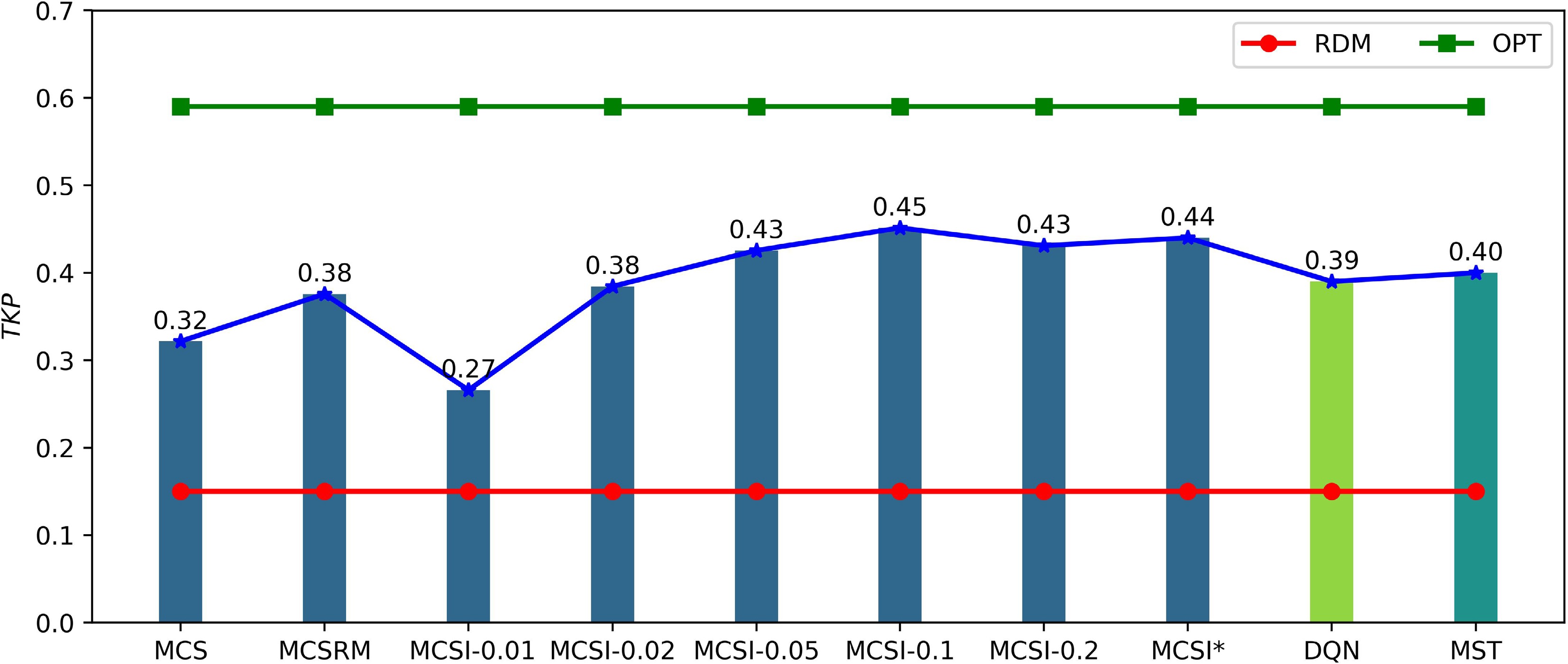
Figure 3. 

The tracking performance of different methods.

Furthermore, when the planning and prediction methods differ, MCSI* demonstrates superior target tracking performance compared with DQN and MST. The superiority of MCSI* indicates that explicitly modeling the target's behavior and fusing intention inference with Monte Carlo trajectory sampling yields more informative predictions and more effective control than either a fixed predictive model (MST) or a policy learned without explicit intention modeling (DQN).

The methods RDM and OPT do not incorporate trajectory prediction, resulting in their outcomes remaining unaffected by the trajectory prediction techniques applied.

Table 1 summarizes nonparametric significance testing using the Mann–Whitney U test to compare MCS, MCSRM, DQN, and MST against MCSI*. The table reports, for each method, the mean and standard deviation of target tracking performance, together with the U statistic (vs MCSI*) and one-sided p-value. MCSI* achieves the highest mean score, although standard deviations are comparable across methods. For every pairwise comparison, U > 5,000 and one-sided p < 0.05, supporting the directional hypothesis that MCSI* outperforms the baselines. These findings corroborate the superiority of MCSI* and suggest that the gains arise from improved central performance rather than experimental random error.

In a test experiment shown in Fig. 4, at $t $ = 20.0 s, the target is in the FOV of the UAV, as shown in Fig. 4a, the predicted target trajectories are the possible paths from the next node of the target to each goal region (each subfigure below predicts the possible paths from the next node of the target to each goal region), and since the target has just started to move, the predicted probabilities for the target's goal regions are the same, i.e., the size of the yellow circles is the same. Therefore, the predicted trajectories of the target are evenly distributed over the possible paths. As the target continues to move upward, the distribution of the target's goal regions tends to be at the top edge of the environment, as shown in Fig. 4b; at the same time, the predicted target's trajectories are also close to these goal regions. At this stage, it can be seen that the target has escaped from the UAV's FOV through evasive motion. As can be seen in Fig. 4c, d, the UAV is searching for the target, and the target is detected by two ground sensors. On the basis of this information, the UAV updates its prediction of the target's intention and trajectory. Using this prediction information, the UAV captures the target again at $ t $ = 220.4 s, as shown in Fig. 4e. After that, the UAV keeps tracking the target until it approaches its goal region, as shown in Fig. 4f.

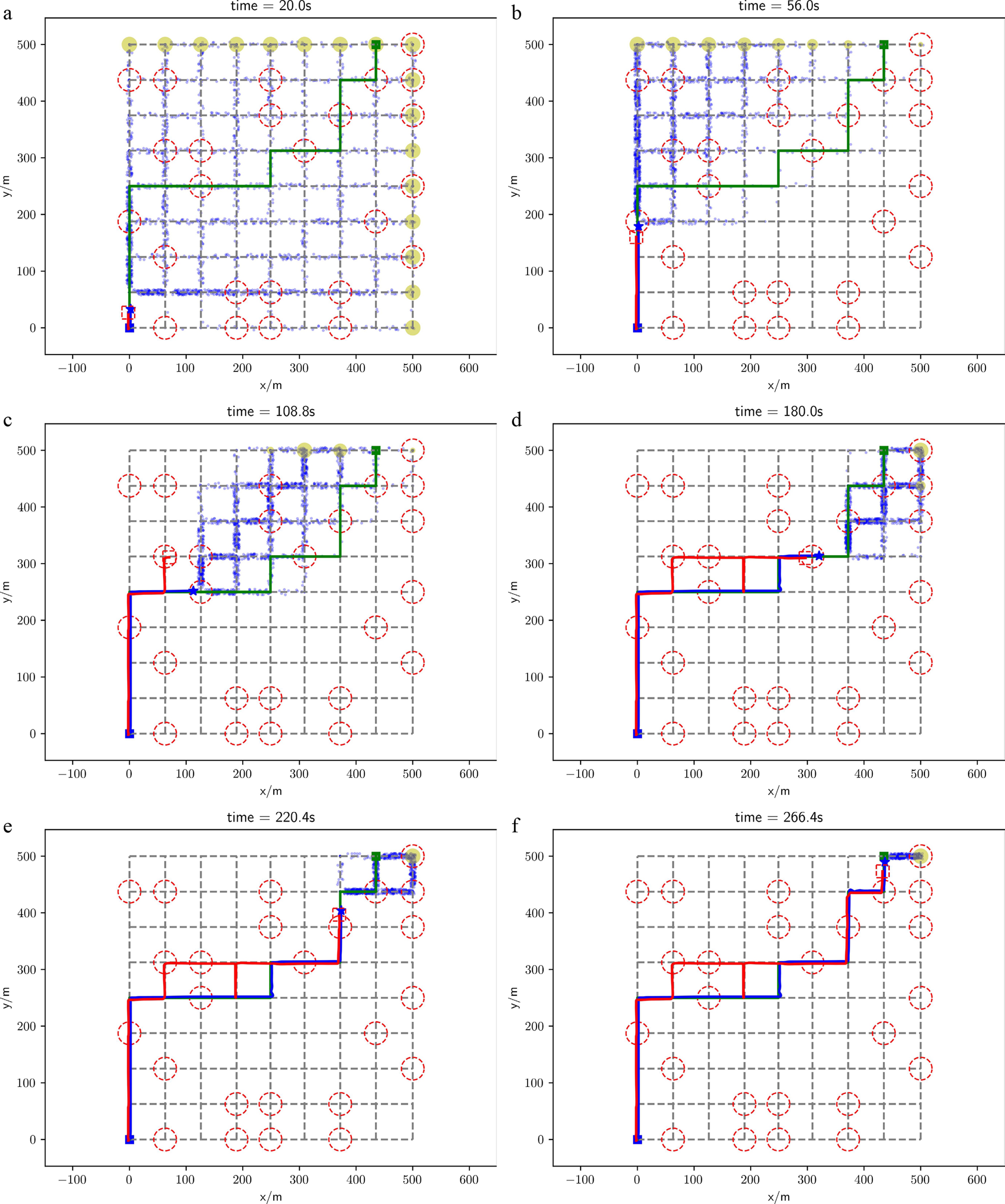
Figure 4. 

Target tracking process in a test experiment. The target prediction method is MCSI*, and the UAV planning method is the MCTS-based planning method. The blue star represents the position of the target, while the dashed red square denotes the FOV of the UAV. The square blue block indicates the target's starting region, and the green square marks the actual goal region of the target. The red dashed circles represent the sensing fields of the ground sensors. The blue solid line illustrates the trajectory of the target, whereas the red solid line depicts the path taken by the UAV. The green solid line shows the planned global path from the target's starting region to its goal region. The blue dots signify the predicted positions of the target, and the yellow circles indicate the potential predicted goal regions of the target, with larger circles representing a higher likelihood of being the target's goal region.

As shown in Fig. 5, when the UAV or ground sensor observes the target moving between two nodes, the value of $ \hat{\beta } $ will be updated. Moreover, during the tracking process of the target, the value of $ \hat{\beta } $ first increases and then decreases. This is because the initial movement trajectory of the target is mainly linear, indicating low uncertainty in the target's behavior, corresponding to a larger $ \hat{\beta } $. However, in the later stage, the movement trajectory of the target is mainly polylinear, indicating high uncertainty in the target's behavior, corresponding to a smaller $ \hat{\beta } $. Finally, based on the observed target trajectory, the value of $ \hat{\beta } $ is approximately 0.125, which is close to the true value of the target behavior parameter ($ \beta $ = 0.1).

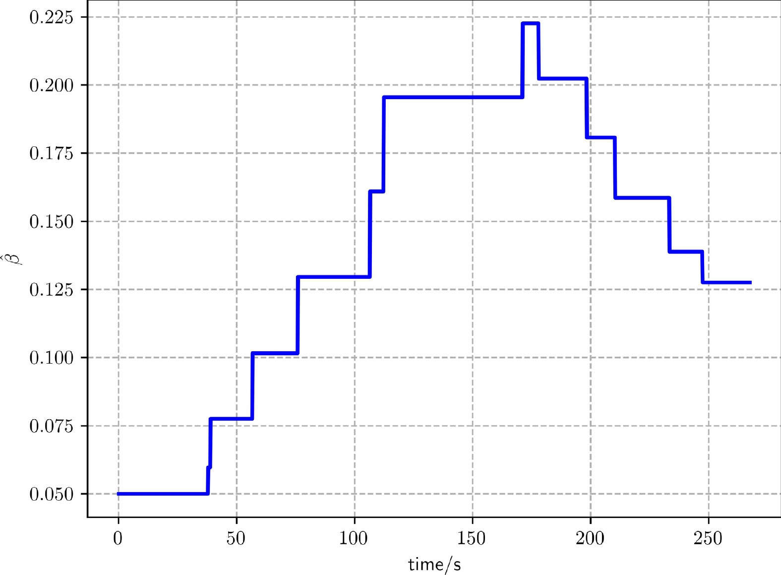
Figure 5. 

The curve of the estimate of the target behavior parameter throughout the tracking process in Fig. 4.

Results with different target's behaviors

In this subsection, we examine the impact of the target's behaviors on target tracking performance. Specifically, we focus on both the global motion behavior and the evasive behavior of the target. The global motion behavior is influenced by the parameter $ \beta $ as described in Eq. (5). A smaller value of $ \beta $ corresponds to greater uncertainty in the target's behavior. The evasive behavior of the target is mainly determined by the target's escape speed $ V_{T}^{e} $ and escape time $ {T}_{e} $ together, and the product of the two represents the farthest distance that the target can escape in one escape cycle. We use the change in the parameter $ {T}_{e} $ to respond to the change in the target's evasive behavior.

As shown in Fig. 6, the target tracking performances under MCSRM, DQN, MST and MCSI* improve as the value of $ \beta $ increases. This enhancement can be attributed to the increased certainty in the target's behavior, which facilitates more accurate trajectory predictions. Additionally, for MCS, as $ \beta $ rises, the target's movement becomes more predictable. Consequently, the assumption in MCS that all goal regions are equally likely becomes less valid, leading to a decline in tracking performance as $ \beta $ increases. The results presented in Fig. 6 further indicate that when the target's behavior exhibits high uncertainty, achieving continuous tracking becomes significantly more challenging.

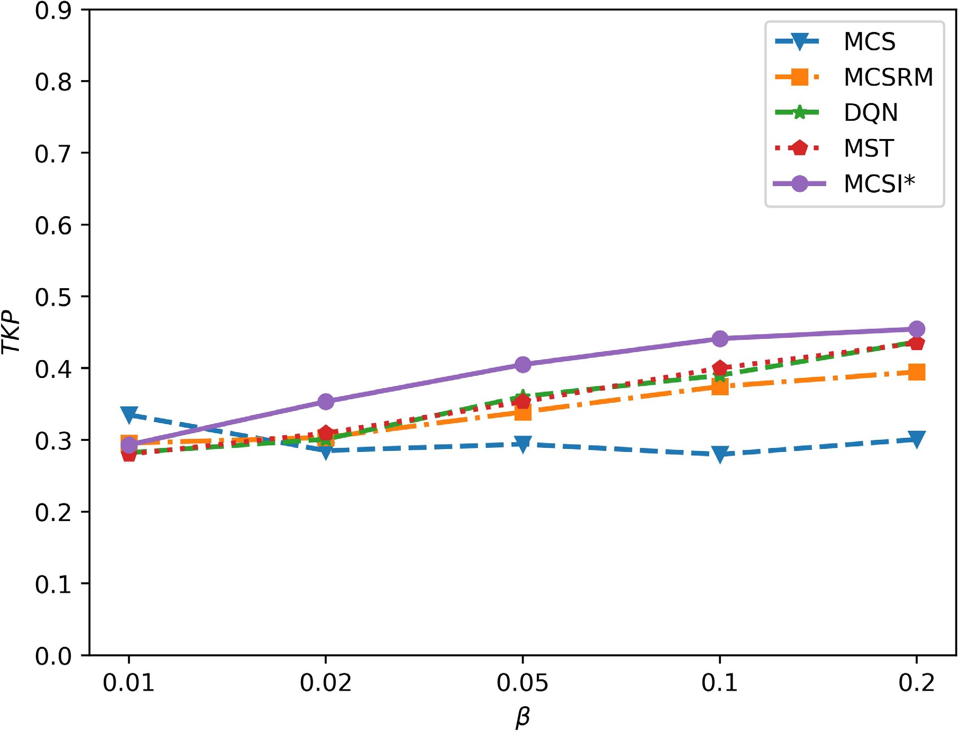
Figure 6. 

The impacts of the target's global motion behavior on tracking performance.

Figure 7 demonstrates the effects of the target's escape time $ {T}_{e} $ on tracking performance. As $ {T}_{e} $ increases, the tracking performance across all methods gradually decline. This trend indicates that as the target's evasive capability strengthens, maintaining continuous tracking becomes increasingly difficult. The results highlight the challenges posed by longer escape times, emphasizing the need for enhanced tracking strategies to cope with more evasive targets.

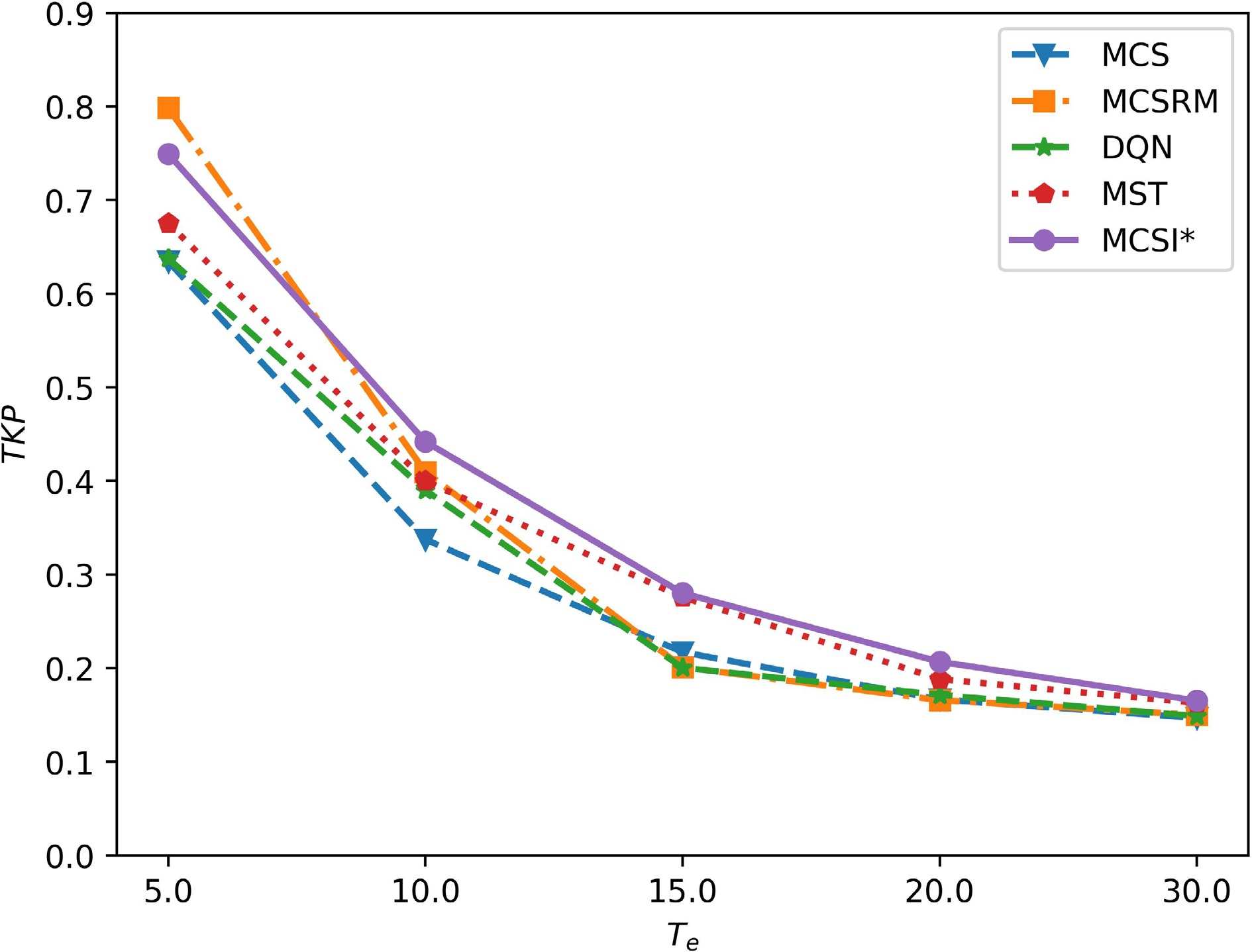
Figure 7. 

The impacts of the target's evasive behavior on tracking performance.

Moreover, when ${T}_{e}$ = 5 s, the target exhibits weak escape behavior, and MCSRM demonstrates superior target tracking performance. This indicates that when the target moves outside the FOV of the UAV, it is frequently possible for the UAV to reacquire the target by tracking its trajectory in the direction of its escape. When ${T}_{e}$ = 30 s, the target displays pronounced escape dynamics, and the tracking outcomes across methods converge, failing to sustain effective tracking. This suggests that one UAV is insufficient, motivating either multi-UAV deployment or other approaches for persistent surveillance.

It should be noted that in the current simulations, the target's global motion is generated using the same exponential-distance-based transition rule that the prediction model assumes. This deliberate consistency allows us to isolate the contributions of intention inference and online parameter estimation. In practice, however, a mismatch between the assumed and actual target behavior model is inevitable. A severe structural mismatch, such as when the target follows a fundamentally different decision rule or uses deceptive strategies, would undermine the validity of the likelihood model and degrade the accuracy of intention inference. Addressing such scenarios through data-driven behavior modeling that relaxes strong parametric assumptions remains an important direction for future work.

Sensitivity analyses

In this subsection, we explore the impact of key parameters ($ N_{p}^{MCTS} $, $ {H}_{p} $, $ \gamma $) in MCSI* on tracking performance. The results are illustrated in Fig. 8. As shown, increasing $ N_{p}^{MCTS} $ from 50 to 400 yields monotonic improvements, but the marginal gains diminish once $ N_{p}^{MCTS} $ exceeds 200. Because the runtime grows substantially with $ N_{p}^{MCTS} $, $ N_{p}^{MCTS}=200 $ offers a favorable balance between accuracy and computational cost. Varying $ {H}_{p} $ and $ \gamma $ produces an inverted U pattern: Performance initially improves as deeper rollouts and greater emphasis on future rewards enrich planning, but declines at higher values because of accumulating prediction uncertainty and increased sensitivity to long-horizon model errors. Thus, moderate values of $ {H}_{p} $ and $ \gamma $ provide the best trade-off between foresight and reliability. Across the explored parameter ranges, the tracking performance varies within 0.41–0.445, indicating low sensitivity overall and demonstrating that MCSI* is robust to reasonable parameter choices.

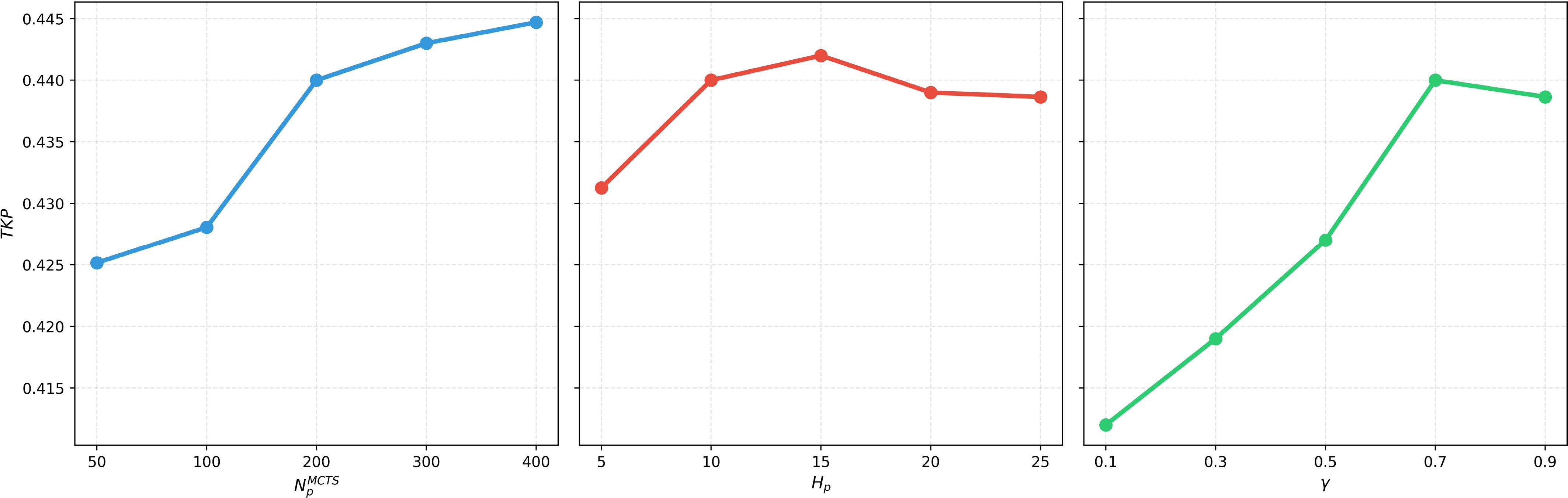
Figure 8. 

The impacts of the key parameters on tracking performance.

Operating cost and complexity analyses

The algorithm's operating cost and complexity are primarily determined by three core components: Intention inference, trajectory prediction, and MCTS-based planning.

Intention inference

The Bayesian update of the target's intent (Equation (4)) involves calculating the posterior probability $ P({g}_{T}|x_{T}^{0: t}) $ for all candidate goal regions. If there are $ G $ potential goal regions, each update requires $ O(G) $ operations to update the posterior. The real-time estimation of the behavioral parameter $ \hat{\beta } $ adds $ O(1) $ per trajectory observation, as it only depends on the latest three nodes traversed by the target. Hence, intention inference imposes an extremely light computational burden.

Trajectory prediction

The MCSI method samples $ N_{T}^{MC} $ trajectories, with each sample generated by simulating path selection from the current node to a goal region. Let $ L $ denote the average number of node transitions along such a trajectory (expected to be on the order of tens of steps for a 9 × 9 grid). The overall complexity is $ O(N_{T}^{MC}\cdot L) $. With $ N_{T}^{MC} $ = 100, this amounts to a few thousand node-transition sampling operations, which is computationally inexpensive.

MCTS-based planning

The MCTS planner is invoked when the target is outside the UAV's FOV. Each planning cycle runs $ N_{p}^{MCTS} $ iterations. In a single iteration, the selection step traverses the tree to a depth at most $ {H}_{p} $, the expansion step adds a node in $ O(1) $, the simulation step generates a goal-conditioned trajectory of length $ {H}_{p} $ and evaluates the cumulative detection reward, and the backpropagation step updates statistics along the path. Hence, the per-iteration cost is dominated by the simulation phase and is $ O({H}_{p}) $. The total per-planning-cycle complexity is therefore$ O(N_{p}^{MCTS}\cdot {H}_{p}) $.

In summary, the computational complexity of the algorithm is primarily dominated by trajectory prediction and MCTS-based planning, with the overhead incurred by intention inference being negligible. In the simulation environment, a single algorithm's operating step can be completed in less than 20 ms on a standard laptop (CPU: AMD Ryzen 7 7840HS; Memory: 16.0 GB, 6,400 MT/s), which demonstrates the real-time applicability of the overall framework.

The results presented above indicate that both intention inference and online estimation of the behavioral parameter can materially enhance tracking performance. Nevertheless, in operational settings with adversarial targets, reliable behavioral models are difficult to obtain. Moreover, targets may act nonrationally, limiting the accuracy of intention models and making intention prediction particularly challenging.

A viable strategy for addressing this issue involves using deep neural networks to model the behavior of the target, with real-time updates to the model parameters according to the observed trajectory of the target. However, a significant challenge in this approach is the development of an efficient method for rapidly updating the neural network parameters. Moreover, as the uncertainty surrounding the target's behavior increases, accurately predicting its intentions and trajectory becomes more complex, which hinders the ability of a single UAV to maintain continuous tracking. In contrast, the utilization of multiple UAVs offers a promising solution. On the one hand, multiple UAVs have greater detection capabilities and can achieve rapid search and detection within the environment to quickly discover the target; on the other hand, coordinated multi-UAV deployments enable deliberate interaction with the target, reducing behavioral uncertainty, which, in turn, simplifies intention inference and supports persistent tracking.

This study explores the challenge of UAV-based tracking for a target that exhibits evasive behavior in an urban environment. Unlike previous research, the focus here is on targets that can evade tracking through rapid acceleration. To enhance the UAV's ability to locate an escaped target swiftly, the planning process is informed by inferring the target's intentions and predicting its trajectory. Additionally, the target's behavioral parameter is updated online from its observed motion. The simulations indicate that intention inference effectively steers the UAV's planner, and online parameter estimation yields substantial gains in tracking performance. Nonetheless, as the target's evasive capabilities increase, maintaining continuous tracking becomes increasingly challenging for a single UAV. Moreover, accurately modeling and estimating the target's behavior in real time presents practical difficulties. Future research will focus on developing cooperative tracking strategies involving multiple UAVs and constructing behavior models based on real-time trajectory data from the observed target.