Physical information embedded dual residual network for UAV actuators fault diagnosis

UAVs serve as low-altitude economic carriers and have attracted extensive attention against the backdrop of rapid advances in engineering and artificial intelligence^[1]. Fixed-wing UAVs, which are characterized by high endurance and heavy payloads, have become key components in logistics, surveying, and mapping scenarios. SF Express has developed a fixed-wing UAV specifically for the logistics industry^[2]. The performance of such aircraft depends on the precise control of their actuators to maintain stable attitudes and trajectories; once actuator faults occur, the mission success rate decreases to nearly zero. Therefore, the accurate estimation of the fault states of fixed-wing UAV actuators is an urgent research issue^[3−5].

Two fault diagnosis approaches have been introduced: model-based and data-driven approaches. Model-based methods detect faults by establishing mathematical models of the target UAV system and comparing model-predicted responses with actual system measurements. These methods make use of prior physical knowledge and usually provide good interpretability and diagnostic reliability^[6]. Early studies mainly relied on linear models, such as Kalman-filter-based approaches for UAV sensor and actuator fault diagnosis^[7]. However, UAV systems are inherently nonlinear, and linear models are often insufficient for describing complex flight dynamics under varying operating conditions^[8]. To address this issue, nonlinear model-based methods, including nonlinear observers, equivalent-space methods, and adaptive robust fault estimation techniques, have been developed^[9]. Nevertheless, as UAV platforms and mission scenarios become increasingly diverse, establishing an accurate high-fidelity model for each specific UAV remains difficult and labor-intensive.

With the development of machine learning, data-driven fault diagnosis methods have gradually become an important research direction. These methods can automatically extract fault-related features from flight data and reduce the dependence on manual feature engineering^[10−15]. For spatial feature extraction, one-dimensional convolutional neural networks and depthwise separable convolution have been applied to fault diagnosis tasks^[16,17]. For temporal modeling, LSTM, BiLSTM, and attention-based recurrent models have shown advantages in capturing sequential fault features^[18,19]. In multisensor systems, graph convolutional networks and spatiotemporal graph neural networks can exploit sensor relationships to improve diagnostic robustness^[20,21]. More recently, Transformer-based models have demonstrated strong capability in long-sequence modeling, and hybrid architectures such as CNN-LSTM and GNN-Transformer models have become effective solutions for complex fault diagnosis tasks^[22].

Despite these advances, existing data-driven methods still face several limitations in UAV actuator fault diagnosis. Most deep learning models rely heavily on data-derived representations and fail to explicitly incorporate the physical operating rules of UAV systems. As a result, physical constraints, state-transition relationships, and fault-induced dynamic deviations are often ignored. For example, although Transformer-based and time-series models such as MTCL-UAV, TimesNet, and PatchTST can extract temporal features, they may confuse true fault characteristics with noise-induced fluctuations when physical constraints are absent^[23]. This issue becomes more serious under sensor noise, environmental disturbance, and measurement uncertainty, especially when fault features are weak or multiple fault modes coexist.

Embedding physical information into deep learning models provides a promising way to address these limitations. UAV motion equations, attitude dynamics constraints, and state-transition relationships describe the fundamental operating mechanisms of the aircraft. By introducing such physical information into feature extraction, the model can better highlight physically consistent fault-related deviations while suppressing irrelevant noise. This helps improve the discriminability, robustness, and interpretability of fault features, especially under complex and noisy flight conditions.

To address the above problems, a fault diagnosis network named PIEDRN is proposed. This approach combines normal and fault data to deeply embed physical information, thereby effectively mitigating the effect of sensor noise on fault diagnosis. Our contributions are listed below.

(1) A physical information-embedded dual residual network is proposed for UAV actuator fault diagnosis. By introducing UAV motion equations and state-transition residuals, the proposed model enhances fault-sensitive features and improves robustness against noise interference.

(2) A cross-attention fusion mechanism is designed to integrate raw temporal features with physics-guided residual features, enabling the model to capture complementary fault information from multichannel flight data.

(3) An adaptive loss Transformer classifier was designed to enhance the traditional Transformer network’s capability to capture long-sequence fault features in data. This effectively improves the accuracy and robustness of fault diagnosis in noisy conditions.

(4) The experimental results demonstrate that PIEDRN comprehensively outperforms the existing methods on both the ALFA and FW-UAV datasets and maintains high accuracy and stability, especially under noisy conditions. Ablation and interpretability analyses further verify the effectiveness of physical information embedding.

The remainder of the article is organized as follows. In the section "Methodology", we discuss the methodology and architecture of PIEDRN. The section "Experimental design" presents a comparative experimental analysis and the results that were obtained across the two datasets. Finally, we conclude the paper.

The proposed method unifies physical-equation residuals and data-driven state residuals into a physics-guided representation learning framework. During flight, UAVs can still fly normally even in the presence of minor faults. However, if these faults accumulate further, serious accidents may occur. In this study, a new network architecture for UAV fault diagnosis is proposed. The network consists primarily of a dual residual enhanced network and an adaptive loss Transformer classifier module. The overall network architecture is shown in Fig. 1. For clarity, vectors are represented by bold lowercase letters, matrices by bold uppercase letters, and scalars by italic symbols throughout this paper.

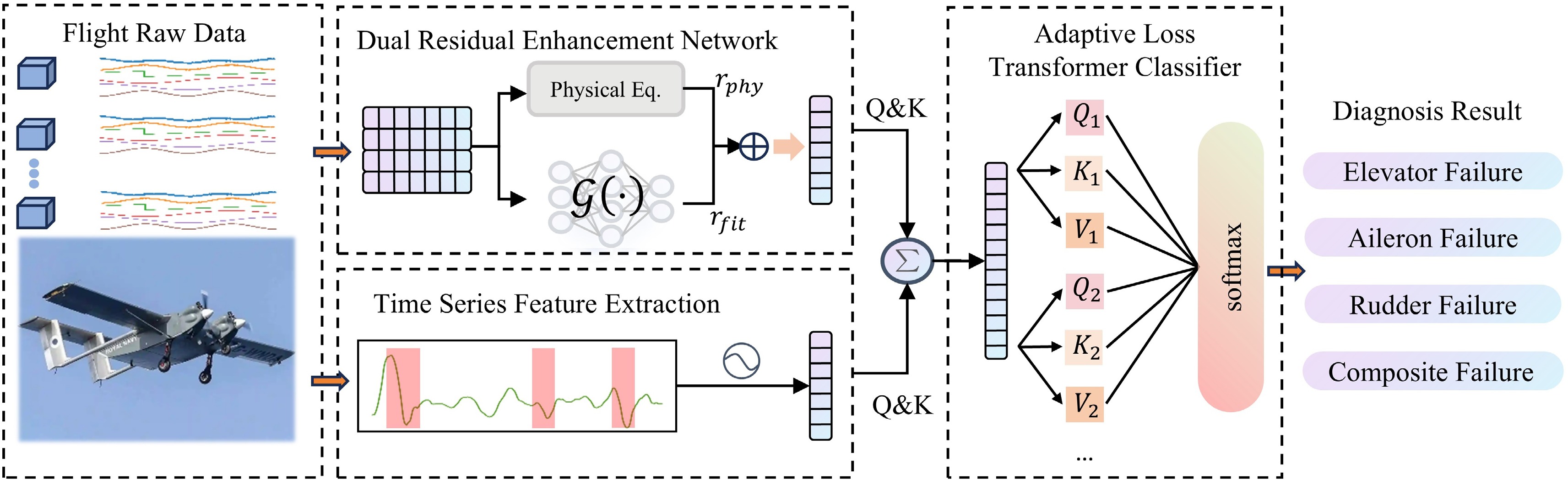
Figure 1. 

Overall network architecture of the PIEDRN fault diagnosis model.

Dual residual enhancement network

The actuator faults considered in this study mainly include control-surface effectiveness degradation and abnormal actuator responses. For a fixed-wing UAV, an actuator fault changes the actual control-surface deflection relative to the commanded deflection. This mismatch alters the aerodynamic forces and moments generated by the aircraft, which subsequently affects the attitude response, angular motion, acceleration, and velocity evolution. Under healthy conditions, the measured motion states are approximately consistent with the kinematic propagation and nominal state-transition relationship. In contrast, when actuator effectiveness degrades, the measured states deviate from the expected evolution because the actual aerodynamic response no longer matches the nominal control response. Therefore, such faults can be characterized by: (1) increased inconsistency between propagated and measured velocity states; and (2) increased deviation from the learned normal state-transition dynamics. These two characteristics motivate the physical residual branch and state-fitting residual branch of PIEDRN, respectively. The dual-residual design is thus intended to capture complementary fault-sensitive deviations from both explicit kinematic constraints and implicit nominal flight dynamics.

During data preprocessing, we typically apply physical models such as the Brownian motion model to perform operations such as noise reduction. These operations demonstrate the potential of physical information in data analysis. In this section, we introduce the proposed PIEDRN model. The network mainly consists of a dual residual enhancement network (DRN) and an adaptive loss Transformer classifier. The design is illustrated in detail in Fig. 1.

Physical equation residual line

The physical residual branch is designed based on the kinematic relationship between the measured UAV velocity and the velocity propagated from inertial measurements. Considering that actuator faults primarily affect attitude and acceleration, such abnormalities accumulate in velocity prediction and manifest as inconsistencies between predicted and measured states. Thus, residual signals from the physical motion equation provide fault-sensitive information while suppressing random sensor fluctuations. The model is derived under standard rigid body flight assumptions, i.e., the UAV is modeled as a rigid body, neglecting aerodynamic elastic effects, structural deformation, and high-frequency vibration dynamics. Since the full rotation matrix is employed for coordinate transformation, no small angle approximation is required. This is consistent with the datasets, which mainly consist of normal flight and moderate maneuvering conditions. Consequently, the kinematic propagation model is applicable to the operational conditions represented in the considered datasets.

For practical implementation, we assume that the sampling interval $ \Delta \mathrm{t} $ is sufficiently small and that the inertial measurements are synchronized with the flight-state measurements. The body-frame acceleration is transformed into the navigation frame through the rotation matrix $ Rt $, and gravity compensation is subsequently performed. Under normal flight conditions, the predicted velocity remains close to the measured velocity. In contrast, actuator faults introduce abnormal aerodynamic responses and control deviations, causing the residual magnitude to increase. This principle is based on the difference between the dynamic equation of an unmanned aerial vehicle and its actual measured motion state. The predicted velocity is defined as:

where, $ v_t\in R^\nVDash$ denotes the measured velocity, $ \hat{v_t}\in R^\nVDash$ denotes the predicted velocity, $ a_t^b\in R^\nVDash $ denotes the body-frame acceleration, $ R_t\in SO\left(3\right) $ denotes the rotation matrix, $ {\bf{g}}\in R^\nVDash $ denotes the gravity vector. The physical residual is then defined as:

Unlike conventional residual generators that require an accurate system model, the proposed residual is obtained from a simplified physical propagation equation and measured flight states. Consequently, it is computationally efficient and can be directly calculated from onboard sensor data. Since actuator faults alter the force and moment balance of the UAV, their effects are reflected in the mismatch between the predicted and actual motion states, making the physical residual a meaningful indicator of abnormal behavior. Thus, the residual vector is:

where, $ r_{t,i}^p $ represents the residual along each axis.

State fitting residual line

Although the physical motion equation captures first-order kinematic inconsistencies, it cannot fully describe the nonlinear state-transition characteristics of UAV dynamics. To further exploit latent physical information, a state-fitting residual branch is introduced. This branch learns the nominal state evolution pattern from normal flight data and detects deviations caused by actuator faults through prediction errors. The strategy of fitting residuals for the state equation involves embedding the state equation of the target unmanned aerial vehicle into a multilayer perceptron (MLP), thereby deeply integrating physical laws and data-driven methods. The system dynamics of the UAV in its normal flight state can be expressed as follows:

where, $ x_{t} \in {\mathbb{R}}^{n} $ represents the state vector, $ u_{t} \in {\mathbb{R}}^{m} $ represents the control input, and $ w_t $ represents process noise. A neural network $ \hat{f}\left(\cdot\right) $ is used to approximate system dynamics:

The neural network is pretrained using only normal-flight data, where the target output is the measured next-step state $ x_{t+1} $. The network parameters are optimized by minimizing the mean squared prediction error between $ x_{t+1} $ and $ \widehat{x_{t+1}} $. In this way, the learned model approximates the nominal state-transition function of the UAV. During inference, unseen fault conditions lead to larger prediction discrepancies because the observed state evolution no longer follows the learned normal-flight dynamics. The state residual is defined as:

During normal operation:

Under fault conditions, deviations occur:

where, $ \hat{f}\left(\cdot\right) $ denotes the neural-network approximation of the physical state transition function $ f\left(\cdot\right) $. The state residual can be interpreted as a data-driven approximation of the model mismatch. Under healthy operating conditions, the learned transition model accurately predicts future states and the residual remains small. When actuator effectiveness degrades, or abnormal control responses occur, the state-transition pattern deviates from the nominal dynamics, resulting in a noticeable increase in residual magnitude. Therefore, the state residual serves as a complementary fault-sensitive feature to the physical equation residual.

Cross-attention fusion module

When extracting physical information from the original training data, appropriate methods need to be used to achieve deep interactions between the extracted physical information and the original data. We construct a paired query-key approach to accomplish deep fusion between the original information and the physical residual information. We treat the hidden states that are obtained from the temporal features extracted from the original data as query vectors, whereas the physical residual information serves as the key vectors. By calculating the temporal similarity weights between the queries and keys ($ Q \& K $, respectively), we achieve focused attention on the physical residual information. First, we construct the three projection matrices that are required for cross-attention:

where, $ Q_{cross}\in R^{\left(T\times d_k\right)} $, $ K_{cross}\in R^{\left(T\times d_k\right)} $, and $ V_{cross}\in R^{\left(T\times d_k\right)} $ represent the query vector, key vector, and value vector, respectively. $ {H}_{x} $ and $ {H}_{r} $ denote the hidden state matrices of the original data and physical residual data after the temporal feature extraction process, respectively. $ {W}_{Q}^{\text{cross}} $, $ {W}_{K}^{\text{cross}} $, and $ {W}_{V}^{\text{cross}} $ represent the query projection weight matrix, key projection weight matrix, and value projection weight matrix, respectively. $ V^{cross} $ is the value vector. The distribution of the attention weights is as follows:

where, $ d_k $ represents the dimensionality of the query and key vectors. By adjusting $ d_k $, numerical stability is maintained to ensure a reasonable attention weight distribution. The mixed feature representation is as follows:

Adaptive loss Transformer classifier

On the basis of the acquired feature representations, we use an adaptive loss Transformer classifier to extract the key fault features within the temporal dependencies, ultimately yielding probabilities for different fault modes. The fused feature $ Z_t $ is projected into a unified space:

The motivation of the adaptive loss function is to balance physical feature preservation and classification discrimination during different training stages. In the early stage, the residual-enhanced features generated by the dual residual network may not be fully aligned with the Transformer feature space. Therefore, a relatively larger feature-consistency weight encourages the classifier to preserve physically meaningful residual information and prevents the network from relying only on label-driven correlations. As training progresses, the optimization focus should gradually shift toward classification discrimination, so that inter-class separability can be further improved. This design follows a multi-objective optimization strategy, where the feature-consistency loss acts as a physical information regularization term, and the classification loss provides supervised fault-discrimination guidance. The adaptive coefficient $ \alpha(\tau) $ dynamically adjusts the relative importance of these two objectives, enabling the model to achieve a better trade-off between physics-guided representation learning and fault classification accuracy. The specific formula is as follows:

The first term is the feature consistency loss:

where, $ z_t^{ref} $ denotes the reference feature obtained from the residual-enhanced encoder. The second loss is the classification loss, which increases the separability of the features:

where, $ y_c $ and $ \widehat{y_c} $ denote the ground-truth label and predicted probability of class c, respectively. The weighted calculation method is defined as follows:

where, $ \tau $, $ \tau_{max} $, $ \eta $, and $ \beta $ denote the current epoch, the total number of epochs, and the hyperparameters, respectively. $ \sigma\left(\cdot\right) $ is the Sigmoid. In this formulation, $ \eta $ controls the transition rate between feature-consistency learning and classification-oriented learning, while $ \beta $ determines the initial weighting bias. A larger $ \eta $ accelerates the shift toward classification optimization, whereas $ \beta $ adjusts the initial contribution of the physical feature-consistency constraint. The values of $ \eta $ and $ \beta $ were selected based on validation-set performance through Bayesian optimization to achieve a balanced trade-off between representation learning and fault discrimination. $\eta<0$ controls the decay rate of the feature-consistency weight. The feedforward network dimension is set to four times $ d\_model $, with key parameters such as attention heads and network layers automatically optimized via the Optuna framework. After feature encoding by the Transformer, the output from the final time step is sent to a fully connected layer and mapped to the fault category space. The softmax function outputs prediction probabilities, thereby efficiently accomplishing both single- and multi-fault identification.

Training strategies and optimization

The training procedure comprises two stages. In the first stage, the dual residual network was trained exclusively on normal-flight data to learn nominal physical and state-transition characteristics. After convergence, the residual-enhanced features were generated and combined with raw flight data through the cross-attention fusion module. In the second stage, the complete PIEDRN framework was fine-tuned end-to-end using both normal and fault samples, allowing the Transformer classifier to jointly optimize feature representation and fault discrimination. The UAV fault diagnosis procedure of the PIEDRN network is shown in Fig. 2. For all experiments, the Adam optimizer was employed for parameter optimization. The maximum number of training epochs was set to 200, and early stopping was triggered when the validation loss did not improve for 20 consecutive epochs. The batch size was fixed at 64. To improve reproducibility, all experiments were repeated using the same random seed (seed = 42). Model selection was performed according to the best validation accuracy.

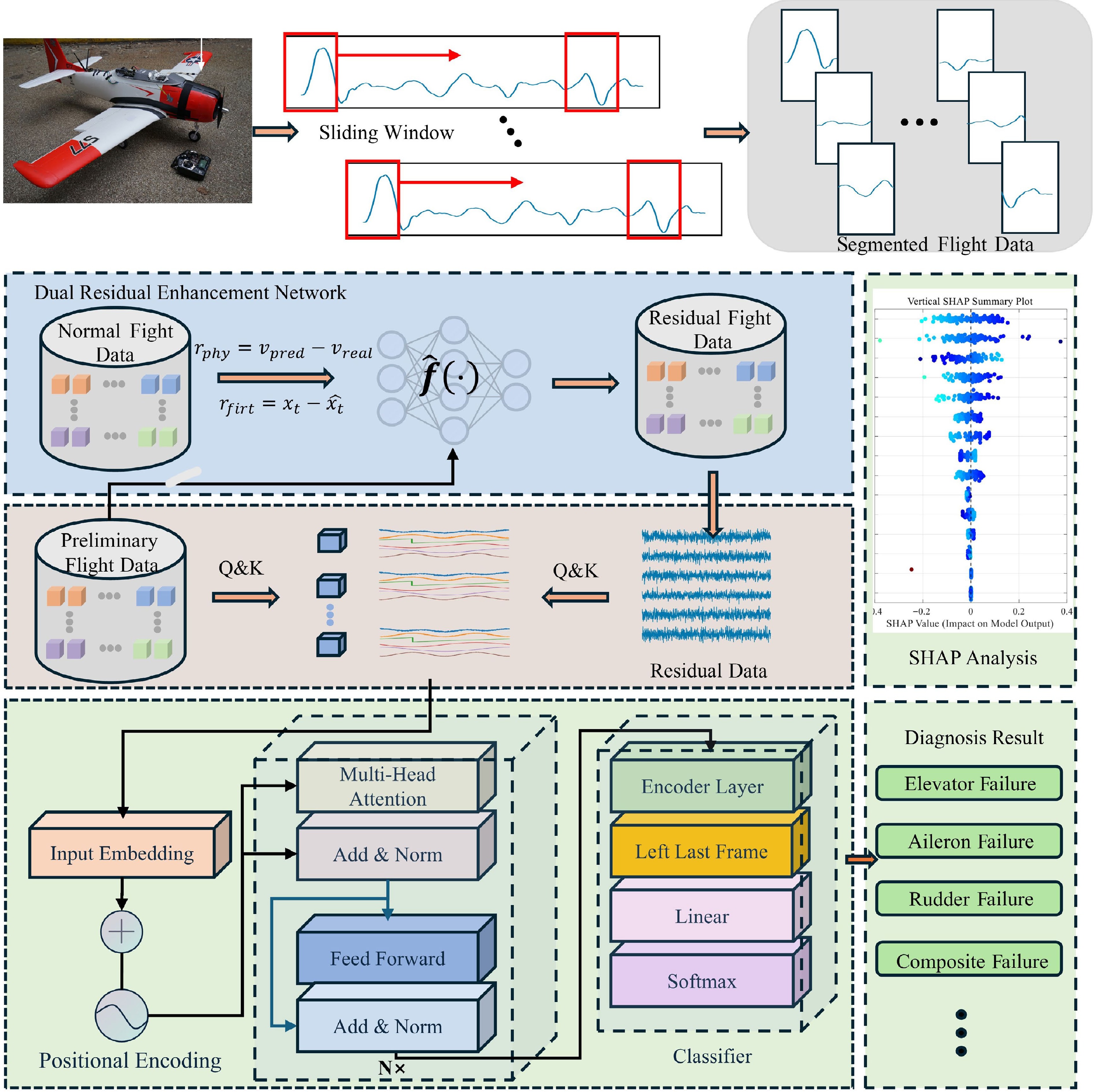
Figure 2. 

UAV fault diagnosis procedure based on the proposed PIEDRN model.

Key hyperparameters (e.g., hidden layer dimensions, number of attention heads, dropout rate, and learning rate) are automatically optimized using Bayesian optimization algorithms within the Optuna framework. The Optuna framework was configured with 50 optimization trials. The search ranges included: learning rate $ \in [1\times10^{-5}, \;1\times10^{-2}] $, dropout rate $ \in [0, \;0.5] $, hidden dimension $ \in [128,\;512] $, number of attention heads $ \in [2, \;10] $, and number of Transformer layers $ \in [1, \;5] $. Additionally, gradient clipping, a learning rate scheduler, and early stopping mechanisms were applied to prevent overfitting and accelerate convergence. This design ensures stable performance under multiple fault scenarios and noisy environments.

The pseudocode for training and evaluating the PIEDRN is presented in Algorithm 1.

The ALFA dataset was generated and disseminated by a research team from Carnegie Mellon University. It mainly provides real flight data for research on fault diagnosis and isolation as well as anomaly detection for UAVs^[24]. The dataset was collected using a modified Carbon-ZT-28 fixed-wing UAV and involved hardware such as a Holybro PX4 flight control system and an Nvidia Jetson TX2 computer. The dataset includes 47 autonomous flight records, which cover 8 different types of sudden failures. The total flight time includes 66 min of normal flight time and 13 min of post-failure flight data. Moreover, the dataset provides several hours of normal flight status data, including data from scenarios such as autonomous and manual flights.

The FW-UAV dataset was generated by a research team from the University of Toulouse, France. The dataset was collected on a UAV platform with a flying-wing layout using the Paparazzi autonomous driving system and a Raspberry Pi Zero control module^[25−27]. The dataset includes 11 flight records with a total time of more than 6 h, among which approximately 2 h are fault data. The fault types include a decrease in control surface efficiency (such as a 30% decrease in the aileron efficiency level), and the flight data include various flight scenarios (at different wind speeds).

For all datasets, we follow a consistent data partitioning strategy. Specifically, each dataset is randomly divided into training, validation, and test sets with a ratio of 70%/15%/15%. The validation set is strictly separated from the test set to avoid data leakage during hyperparameter optimization. For U1 and U2, the same model architecture is used, while the training strategy is adapted according to the fault complexity (binary vs multi-state faults). All experiments are conducted under identical data preprocessing and evaluation protocols to ensure fair comparison. The dataset partitioning scheme is similar to that of Hu et al.^[23].

In this study, actuator faults are mainly categorized into control-surface effectiveness degradation and abnormal actuator response. Before training, all flight variables were synchronized according to their timestamps and normalized using z-score normalization. A sliding-window strategy was adopted to construct temporal samples, where each sample consisted of $ L $ consecutive time steps and inherited the fault label of the corresponding time interval. Missing values and corrupted records were removed during preprocessing. The same preprocessing procedure was applied to all compared methods to ensure a fair evaluation.

Equipment details and evaluation metrics

The network training platform uses an Intel Core i7-9700K processor and an NVIDIA RTX 2080Ti graphics card, which is equipped with 11 GB of memory. All the algorithms are implemented under the PyTorch 2.0.0 framework. Owing to the adoption of the Bayesian optimization method, the hyperparameters that are used for different datasets are not exactly the same. These include the hidden layer dimensionality (HD), the dropout rate (DP), and the learning rate (LR) of the DRN, as well as the number of attention heads (AH), the hidden layer dimensionality (HD), the number of encoder and decoder layers (LY), the dropout rate, and the learning rate of PIEDRN. The specific parameters are shown in Table 1.

Four sets of core indicators are adopted to comprehensively evaluate the fault diagnosis performance of the tested methods. The accuracy rate (ACC) reflects the overall classification accuracy rate, and the precision (PRE) reflects the reliability of fault alarms. The recall rate (REC) characterizes the ability of the tested model to detect faults. The F1 score comprehensively reflects the average precision and recall rate and is applicable to imbalanced datasets. The complete network configuration, optimized hyperparameters, and evaluation protocol are reported in this paper to facilitate independent reproduction of the experimental results. All methods were evaluated using the same dataset partition, preprocessing procedure, training protocol, and fixed random seed to ensure a controlled comparison. Although the proposed method was consistently validated across multiple datasets, noise levels, and ablation settings, repeated experiments with multiple random seeds and formal statistical significance tests will be conducted in future work to further quantify performance variability.

Baselines

To verify the performance of the proposed model, some deep learning methods were collected as baselines. The following is an overview of the baselines.

(1) MTCL-UAV^[23] is a multiscale Transformer-based model designed for UAV anomaly detection. It adopts a sparse mixture-of-experts architecture, where the Router adaptively selects temporal scales, and a contrastive-learning-enhanced dual attention mechanism captures intrapatch, interpatch, and neighboring patch relationships.

(2) DCdetector^[28] is a time-series anomaly detection model based on contrastive learning. It improves feature discrimination between normal and abnormal patterns, making it suitable for detecting subtle anomalies in complex temporal data.

(3) Anomaly Transformer^[29] is a Transformer-based model specifically developed for time-series anomaly detection. It models temporal dependencies through attention mechanisms and identifies anomalies by measuring abnormal association discrepancies.

(4) TimesNet^[30] is a deep learning model for general time-series analysis. It captures intraperiod and interperiod variations through multiscale temporal modeling and CNN-based structures, but it is relatively weaker than Transformer-based models in capturing global dependencies.

(5) PatchTST^[31] is a patch-based Transformer model for time-series analysis. It divides continuous sequences into patches to enhance local semantic representation and reduce modeling complexity, but it lacks adaptive multiscale modeling for complex UAV flight patterns.

(6) CGAD^[32] is an anomaly detection model that combines causal convolutional and graph convolutional networks. It can capture dynamic patterns in flight data and often performs well in recall, although its complex modeling structure may limit generalization.

Performance comparison

All comparison methods are implemented under the same experimental setting and trained using their recommended configurations. For fairness, we re-implement all baseline models and tune their hyperparameters on the validation set when possible. All methods use identical training/testing splits.

The proposed PIEDRN model demonstrates outstanding performance advantages in the task of detecting faults in UAV actuators, and outperforms the existing methods in terms of all four indicators, as shown in Table 2. The training process of PIEDRN is illustrated in Fig. 3. A comparison of the A1 dataset before and after clustering is shown in Fig. 4. This comparison clearly demonstrates the performance of PIEDRN in feature clustering. The confusion matrices for various subdatasets are shown in Fig. 5. Owing to the limited amount of fault data in some cases, the sampling process cannot guarantee that seven fault types are consistently included. Across various subdatasets, PIEDRN consistently achieves strong classification performance.

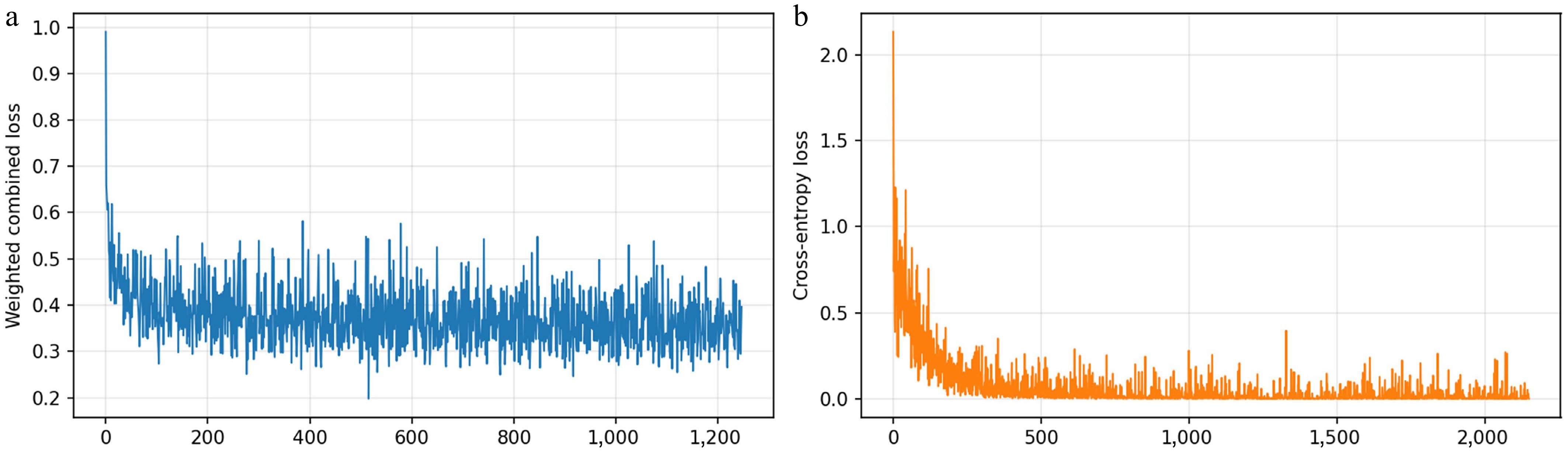
Figure 3. 

(a) Training loss curve for the physical information fusion extractor, and (b) loss decay curve for the adaptive loss Transformer classifier.

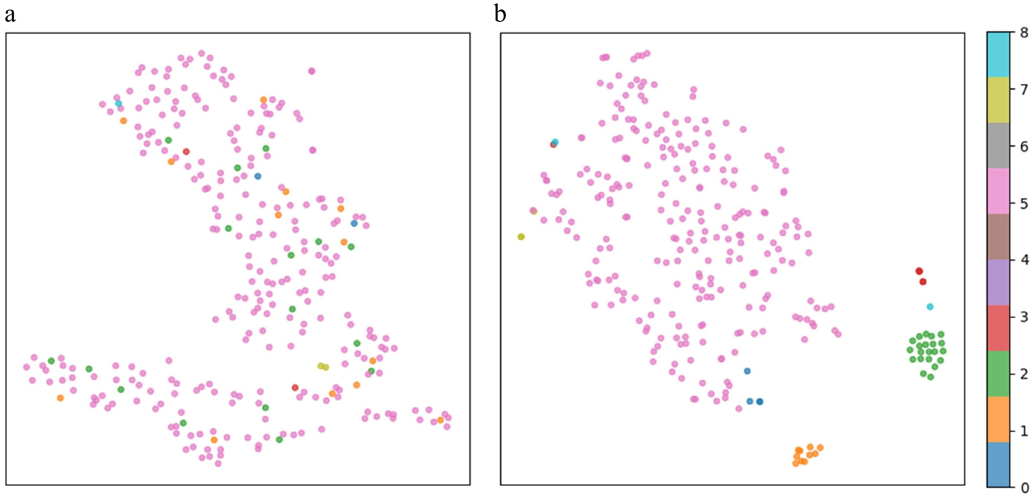
Figure 4. 

(a) t-SNE plot without feature clustering, and (b) t-SNE plot after feature clustering by PIEDRN.

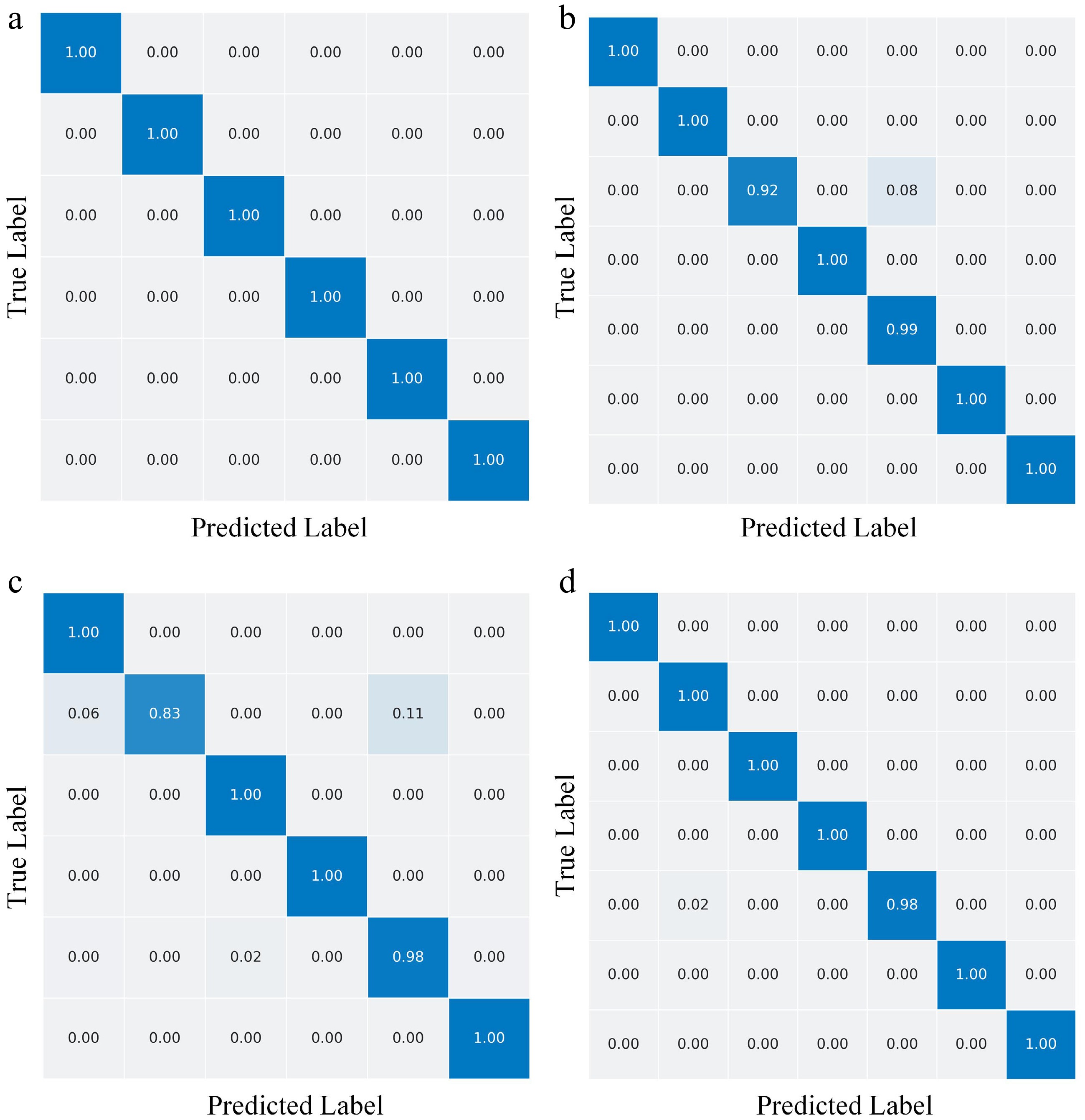
Figure 5. 

Confusion matrix for datasets D1–D4.

The data in Table 2 indicate that the PIEDRN model ranks among the top performers across multiple key metrics, thus demonstrating its superior UAV fault diagnosis capabilities. PIEDRN achieves an average F1 score of 0.9749 and significantly outperforms the second-place MTCL-UAV model. This advantage is intrinsically linked to its partial feature extraction mechanism. The DRN effectively distinguishes noise from actual fault signals and amplifies the subtle fluctuations within the data that are indicative of faults. It then feeds the obtained fault states back into the output through an adaptive loss Transformer classifier. We segment the 12-dimensional data that are contained in dataset A1 into 12 channels (Ch), each of which comprises two dimensions. The diagnostic performance of the model across different channels is shown in Fig. 6. Channel 1 demonstrates superior feature representations and is easily diagnosed by the model, whereas on the other channels the model performs poorly. Crucially, the full-channel approach outperforms the single-channel methods across all the metrics, which confirms the ability of our model to integrate multisensor data and extract hidden fault information from multichannel data while mitigating interference.

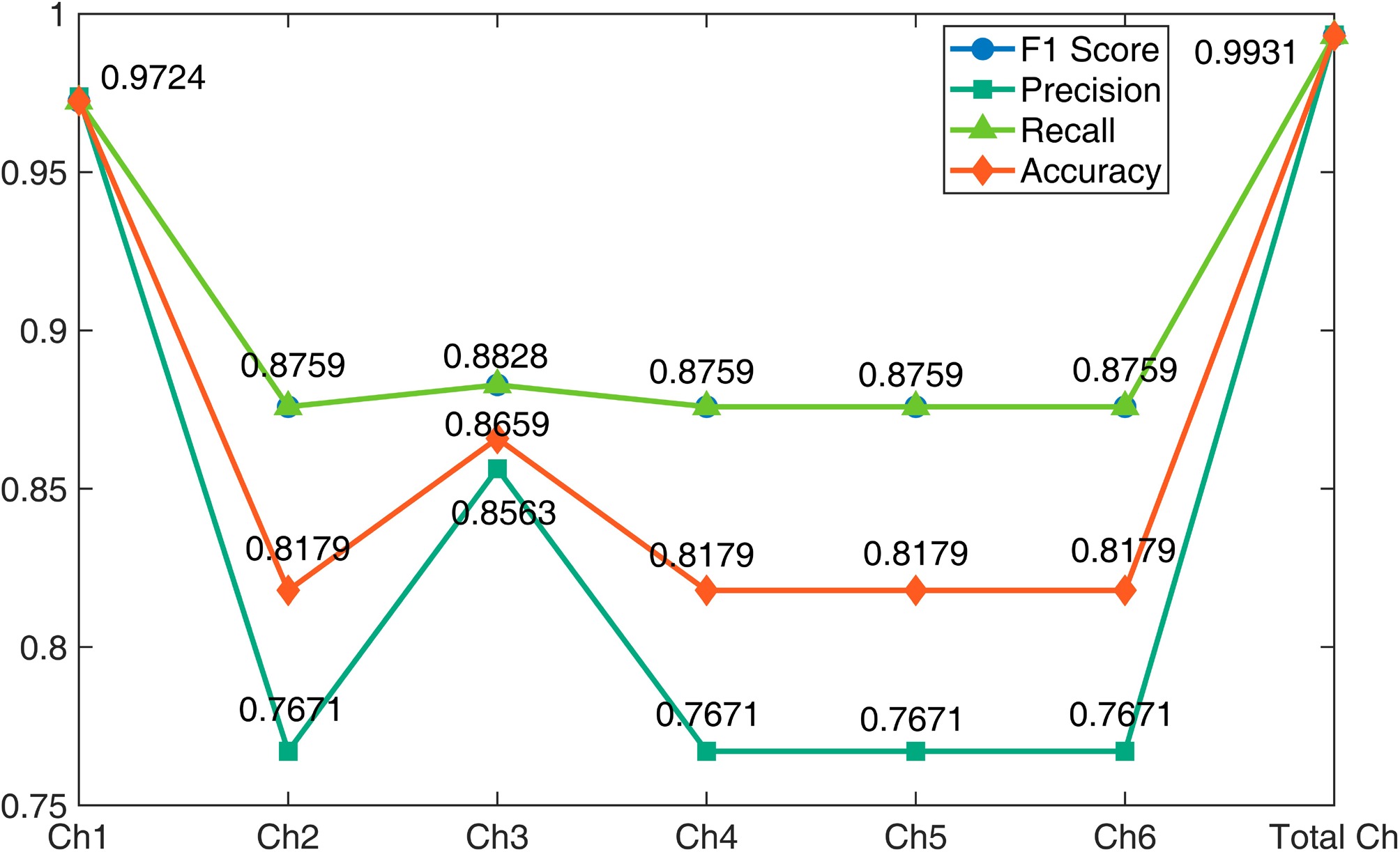
Figure 6. 

Comparison of the classification performances of PIEDRN across different channels.

Across datasets A1–A4, the adaptive loss Transformer classifier also demonstrates outstanding performance. The MTCL-UAV, DCDetector, and anomaly transformer models all incorporate this mechanism. Among them, the MTCL-UAV model uses multiple transformer architectures to jointly learn features and exhibits stronger feature extraction capabilities than a single transformer model does. However, owing to its limited depth in terms of uncovering physical information and the coupling of fault features with noise, its discrimination ability falls short of that of the PIEDRN model. Although models such as TimesNet and PatchTST, which incorporate multihead attention, demonstrate superior time-frequency transformation capabilities and can extract long-term dependencies, their lack of physical constraints results in significantly lower REC and F1 scores on datasets A3 and A4. CGAD attempts to incorporate causal graph structures, but its high modeling complexity limits its generalization ability. Although it achieves 1.0000 recall on A3, its precision decreases to 0.4870. These results demonstrate that in complex UAV systems, fault features are often subtle and easily mixed with noise. Without physical information, the performance of deep learning models significantly degrades.

The comparative results obtained on the FW-UAV dataset are shown in Table 3. The PIEDRN model achieves an average F1 score of 96.36% across datasets U1 and U2 and outperforms methods such as MTCL-UAV (95.68%) and DCDetector (94.58%). This outstanding performance demonstrates the high suitability of the DRN for fault detection in UAVs with flying-wing layouts. The model achieves 98.08% accuracy and recall scores on dataset U2, thus ensuring stable fault alarm triggering without missing hazardous states during multistate UAV failures. PIEDRN achieves superior overall performance across multiple fault modes on dataset U2 because of its focus on integrating physical information extraction with adaptive loss Transformer classifiers. However, the relatively lower performance on U1 may be attributed to its single-fault structure, where physical residual enhancement provides limited additional information. The advantages of PIEDRN become more evident in multi-state and complex fault scenarios.

The core performance advantage of the model stems from its dual residual enhancement design. Unlike methods that rely on multiscale extraction or causal graphs, PIEDRN fundamentally enhances features by embedding physical equations (e.g., motion and state-fitting residuals), which reliably separates fault signals from noise. The subsequent multihead attention mechanism optimally fuses these physics-enhanced features with raw time-series data, capturing discriminative spatiotemporal patterns for multi-fault recognition.

The interpretable SHAP (Fig. 7) indicates that the physical information residual has the highest feature importance. For example, the mean absolute SHAP value for the pitch residual is 0.041, which is significantly higher than that of the original pitch data (0.027). This confirms that physical constraints amplify fault-induced deviations and improve the discriminability of fault-related features. Moreover, the hierarchical contribution of parameters and the strong synergy between control commands and their residuals demonstrate the ability of PIEDRN to capture sensor coupling and provide physically interpretable, high-fidelity diagnostics under noisy and complex fault conditions. The computational complexity of PIEDRN is mainly determined by the Transformer module, with time complexity approximately $ O(T^2d) $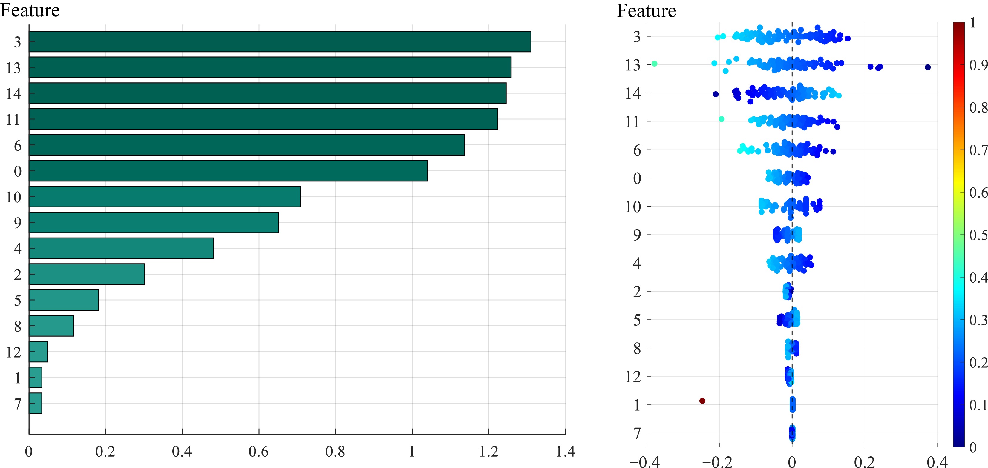. The DRN module introduces only linear overhead, making the method suitable for onboard UAV deployment under moderate sequence lengths.

Figure 7. 

SHAP visualization graph. (a) Mean values of various feature weights, and (b) a scatter plot produced with various feature weights.

Sensitivity and robustness analysis

The hyperparameters of the model are varied on the ALFA dataset, and noise is introduced to test the sensitivity and robustness of the model.

Sensitivity analysis

We also study the influences of the three key parameters of the PIEDRN model on the actuator fault detection results obtained for fixed-wing UAVs. The changes in the parameters and the model detection results are shown in Fig. 8. With respect to the number of PIEDRN layers, the accuracy of the model exhibits a clear inverted U-shaped trend. When the number of layers increases from 1 to 2, the F1 score increases from 97.24% to 99.31%, indicating that a network with more layers has better performance. However, when the number of layers increases to 5, the performance decreases to 97.99%, suggesting that the use of too many layers may lead to model overfitting.

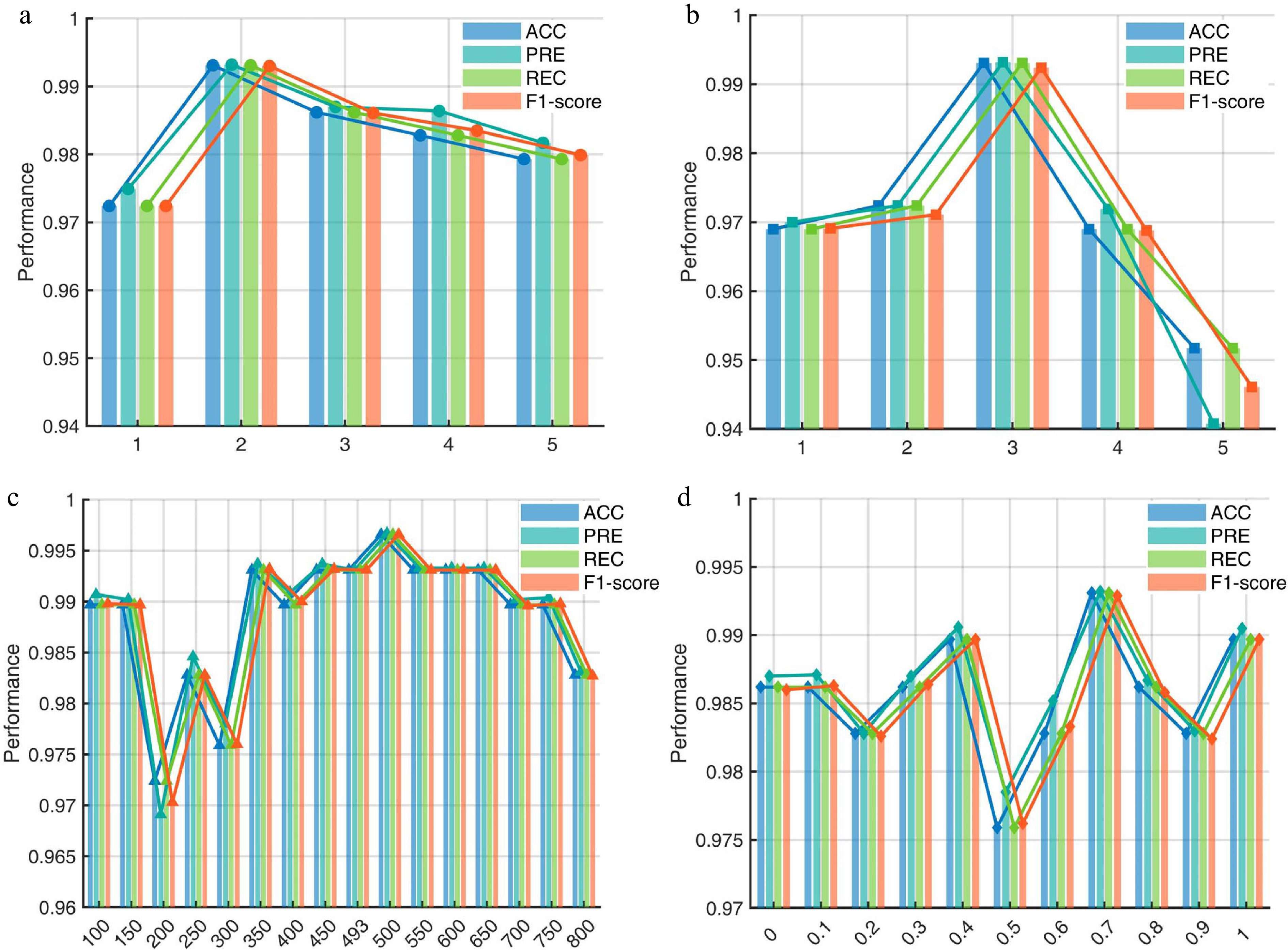
Figure 8. 

Hyperparameter sensitivity change graph: (a) represents the number of stacked layers; (b) is the number of heads contained in PIEDRN; (c) is the number of hidden layers contained in the DRN; and (d) is the size of the weights.

When d_model is 3, the optimal performance is 99.31%. This finding indicates that when d_model is 3, the model can fully utilize the feature information acquired by the DRN and effectively filter the influence of sensor noise. Moreover, when d_model is 5, the performance decreases to 94.61%. This suggests that owing to their excessively high dimensionality, the coupling effects between aerodynamic parameters may affect the prediction of the model. Therefore, in terms of model embeddability, appropriate model dimensions can both ensure the performance of the model and reduce the imposed equipment load.

A sensitivity analysis of the hidden layer dimensionality of the DRN reveals multiple peak characteristics. Within the range from 350 to 650, the model maintains a stable performance level of more than 99.31%, and it reaches its optimal performance at 500 dimensions. This phenomenon indicates that PIEDRN is strongly robust to the capacity of the DRN, but several performance decline points also exist. When the dimensionality increases from 200 to 500, the F1 score increases by 1.25%, whereas it decreases by 0.71% when the dimensionality is between 750 and 800. This finding indicates that the DRN generates the most accurate residuals at 500 dimensions, and the recall rate data also confirm this finding. Therefore, in engineering applications, the optimal configuration of PIEDRN includes 2 stacked layers plus d_model 3 and 500 residual hidden layers. This combination ensures a detection accuracy of more than 99.6% while having lower dimensionality requirements, demonstrating the lightweight advantage of the DRN in engineering practice.

When we analyze the loss weights, we find that different loss weights have different optimal values for indicators such as accuracy. When $ \lambda=0.7 $, the recall rate reaches a peak of 99.31%, which reflects that the model is almost not prone to missed detections. When $ \lambda $ is 0.4, the accuracy is the highest, which is suitable for the low false-alarm rate requirement. Therefore, in engineering practice, the value of $ \lambda $ can be changed according to the needs of the given scenario to obtain the best effect.

Robustness analysis

Noise is independently added to each sensor channel following an additive white Gaussian noise (AWGN) model^[33]. All signals are normalized before noise injection to ensure consistent signal-to-noise ratio (SNR) definitions across datasets. This setup simulates realistic sensor disturbances in UAV flight environments. The noise types and parameter settings are not chosen arbitrarily; they are specifically designed based on typical noise phenomena observed during actual flight tests of our laboratory UAV. Two noise environments with 10% and 20% noise are designed. We also compare our model with several other models evaluated on the same dataset, as detailed in Table 4. The two noise environments are simulated by adding white Gaussian noise to the raw data, with the standard deviations of the noise set to 10% and 20% of the standard deviation of the signal, which results in SNRs of approximately 20 and 14 dB, respectively. The superior performance of our model under noise, as detailed in Table 4, is therefore not only a product of the physics-informed residual extraction process of the DRN and the attention mechanism of PIEDRN but also enabled by the redundancy and complementary information provided by the multichannel data fusion strategy.

The data in Table 4 indicate that the PIEDRN model has strong anti-noise performance. The high accuracy (99.31%) and strong robustness of PIEDRN are attributed to the introduction of the DRN. The DRN filters out environmental noise through physical constraints, thereby enabling PIEDRN to focus on true fault features, which differs sharply from traditional data-driven models. Moreover, the hyperparameter tuning effect of Bayesian optimization reduces the sensitivity of the model to noise, from 99.33% in the noise-free environment to 98.88% in the 20% noise environment, thus avoiding the problem of a significant decrease in the accuracy of models such as the Itransformer in noisy environments.

In contrast, the F1 scores of traditional methods, such as the stacked LSTM model, are reduced to 20% in a 20% noise environment; thus, these methods no longer have practical engineering value. However, owing to the multiple prevention mechanisms of the PIEDRN model, the nonlinear model that is constructed by the DRN achieves noise filtering, and the attention mechanism of PIEDRN performs secondary filtering on the acquired features. In combination with the selection of the optimal hyperparameter combination via Bayesian optimization, the three mechanisms jointly ensure the robustness of the model.

Ablation experiments

To validate the effectiveness of each component module in PIEDRN, we conducted ablation experiments on the physical residual branch, the state residual branch, and the adaptive loss mechanism, respectively. All experiments were conducted under the same data split and training settings. The results are shown in Table 5.

As shown in Table 5, the full PIEDRN model achieved the best performance, with ACC and F1-score reaching 99.31% and 99.30%, respectively. When the physical residual branch was removed, the F1-score dropped to 95.16%, a decrease of 4.14% compared to the full model. This indicates that the physical residuals, constructed based on dynamics equations, can effectively enhance failure-related features and improve the distinguishability between failure and normal states. After removing the state residual branch, the overall F1-score dropped to 95.60%, a decrease of 3.70% compared to the full model. This result indicates that state residuals can effectively characterize the extent to which flight states deviate from normal dynamic evolution patterns, providing supplementary discriminative information for fault diagnosis. Furthermore, when fixed loss weights were used and the adaptive loss mechanism was removed, the model’s performance declined further. The F1-score dropped to 94.63%. Dynamic weighting of the two loss terms strikes an improved balance between feature learning and classification discrimination, leading to enhanced diagnostic performance.

Overall, all three modules made positive contributions to the final performance. Among them, the physical residual branch and the state residual branch together constitute the core feature enhancement mechanism of PIEDRN. The adaptive loss strategy further enhances the model’s ability to learn complex fault features. The results of the ablation experiments validate the rationality and effectiveness of the proposed network architecture design.

In this study, a fault diagnosis framework for UAV actuators is proposed. The network includes a dual residual enhancement network and a Transformer classifier. Through a dual parallel residual enhancement mechanism, it physically enhances raw data by embedding them into physical constraints such as UAV motion equations and state fitting equations. This design generates residual features that describe typical physical characteristics and fully reveal hidden correlations and fault information within the data while preserving the dynamic characteristics of the original time series data. By applying cross-attention mechanisms, the network achieves deep fusion between physically enhanced residuals and original temporal features, thereby providing more recognizable inputs for subsequent diagnosis. Afterward, the mixed features are fed into the Transformer network, which applies its multihead attention mechanism to capture time-space relevance and multifault mode characteristics within long sequences, enabling precise diagnosis across multiple fault statuses. The model achieves over 98% accuracy on both the ALFA and FW-UAV datasets across all the compared metrics and maintains robust anti-interference capability. Future work should focus on incorporating the dynamic equations of the aircraft into the network to improve interpretability and generalizability, thereby promoting the application of physically informed neural networks in the health management of complex systems.