Modeling wheat harvest index using stacking ensemble learning and seeder operational parameters

Among the world's staple foods, wheat is unique as it is a cornerstone crop^[1]. It has been nicknamed 'the king of grains' as it is dominant in most agricultural systems. Iraq alone harvests 1,668,077 ha of wheat per year, with an average yield of 2,546.5 kg/ha^[2]. The nutritional importance of wheat make it fundamental in planning for worldwide food security. It is a diet for over a third of mankind and is responsible for 27% of human protein and calories^[3]. The importance of this crop is immense because it provides raw material for bread, pastries, cookies, pasta, and even the straw is used as animal feed. As the world population is increasing, it has been estimated that it requires increasing its production by 1.6% per year^[4]. This is just another reason why new agricultural management practices are required.

In that context, the Harvest Index (HI), referring to the percentage of cereal yield with respect to total aboveground biomass, constitutes an important agricultural signal; it reflects how effectively plants distribute resources between grain production and vegetative mass construction in crops such as wheat^[5]. For that reason, increasing HI is one of the key targets for breeders and farmers in wheat since it is closely linked with achieving higher yields, coupled with efficient resource utilization, including water and nitrogen^[6,7]. HI is not determined only by genotype and environment but also by agricultural practices^[8]. From among these practices, seed quality and method of seeding assume a lot of importance. Selection of the type of seeder, rate of seeding, and depth of seeding greatly affect the emergence, growth, and yield of wheat, along with HI^[9,10,11]. The accuracy of placing seeds correctly and coming into proper contact with the soil depends on the choice of the seeder. Proper soil-seed interaction and even germination depend on these factors and also lay the foundation for early growth. Modern seeders striking at exact depth and spreading the seeds appropriately can reduce depth variation to a great extent, improve the interaction of seed-soil moisture, encourage uniform emergence, and lead to higher crop vigor^[12,13]. Sowing speed is also considered: too much speed can disallow proper placement of seed, reduced soil contact, low seedling density and growth, which may cause a reduction in yield components and HI accordingly^[10]. Depth of sowing is another major factor; too shallow could expose the seeds to moisture fluctuations and frost, while sowing too deep delays the development of ears and limits branching, hence reducing productivity and yield accordingly^[14,15]. An optimum depth of sowing allows fast and reliable emergence, better plant growth, a higher biomass buildup, and therefore a higher grain yield with improved values of HI^[16,17]. In this way, knowledge of the interaction among the factors of seeder type, sowing speed, and sowing depth to form the wheat HI would be of great importance to exactly determine the practices that would unlock greater yield potential.

Even with improved seeder technology and more subtle control over speed and depth adjustments, the art of predicting actual crop performance remains a knotty problem. There are too many variables: the realms of biology, the atmosphere, and the way farmers tend to their land—these interactions simply cannot be disentangled by the simple experimental methods of the past. This is where machine learning (ML) comes into its own. ML can identify nonlinear correlations within massive amounts of data through innovative algorithms to discern hidden interactions among the ever-increasing number of variables relevant to agriculture^[18,19]. For agriculture specifically, ML relies on soil sensor information, satellite imaging, or phenotyping software to isolate hidden trends to project desirable outcomes like yield or susceptibility to disease^[20,21]. ML algorithms perform exceptionally well by using a diverse array of agricultural, environmental, and climate factors to forecast a HI with strong predictive ability and robustness, even in challenging scenarios^[22,23]. However, although HI is a very important measure for crop efficiency, most research still applies classical statistics. The drawback to these techniques is that, although they can retrospectively interpret discrepancies successfully, they are not capable of representing the non-linear interplay among machine parameters (speed, depth, and type) and prediction outcome. There certainly exists a gap here, where farmers would greatly benefit from 'smart' computer algorithms for adjusting seeder parameters. The proposed study attempts to address the identified gap by conducting an experiment on various operational factors influencing HI; namely seeder type, sowing depth, and sowing speed. The study also designs and implements sophisticated ML algorithms (RF, SVR, and stacking methods) for effectively determining the HI based on machine-related variables.

This study used an integrated experimental and computational approach to evaluate and predict the wheat HI for the IPA 95 variety. The fertilization process followed the best practices in the region for the cultivation of wheat crops. During the seedbed preparation stage, diammonium phosphate (DAP) fertilizer, 100 kg/ha was used in the form of basal fertilizer, and was applied manually. Furthermore, nitrogen fertilizer in the form of urea (46% N), totaling 400 kg/ha, was used in two splits, each 200 kg/ha. The first split was applied manually during the tillering stage, one month after sowing, at the three-leaf stage, and the second split was applied during the booting stage, where spike formation takes place. For irrigation, the method used was surface irrigation. The period between November (sowing) and May (harvesting) was chosen, and irrigation was conducted based on the water requirements of the crops during the stages of growth. The location of the experiment is in a semi-arid region. During the season, the average temperature varies from 12 to 28 °C, and the total rainfall for the season is 150 mm. The quantity of seeds per ha was calibrated, and based on the absence of impurities in the seeds, it was set at 100 kg/ha. The experiment was carried out in a clayey silty soil mixture. Before commencing the experiment, soil samples were collected from the 0−30 cm depth at several random spots across the field using a soil auger. These samples were then combined to obtain a composite sample for conventional analysis. To determine the moisture content, the samples were dried in an oven at 105 °C for 24 h. This gave a soil moisture content of 16%−18%. To determine the pH, the samples were combined and then measured using a digital pH meter after mixing with a 1:1 soil and water solution^[24]. This gave a pH of 7.94. Moreover, the soil organic matter (SOM) was determined using the Walkley-Black chromic acid wet oxidation method, which estimated the SOM content to be 1.37%. Fieldwork consisted of testing three operational variables: seeder type, sowing depth, and sowing speed, using a randomized complete block design (RCBD). Following data analysis to understand which variables were significant, several ML models were used for training and testing of the prediction. The research team constructed RF, SVR, and stacking approaches to uncover nonlinear relationships, thereby improving predictability beyond the capability of traditional linear regression. Their objective was therefore to find the optimal setting of agricultural machinery for maximizing production efficiency. Figure 1 gives an overview of the research methodology.

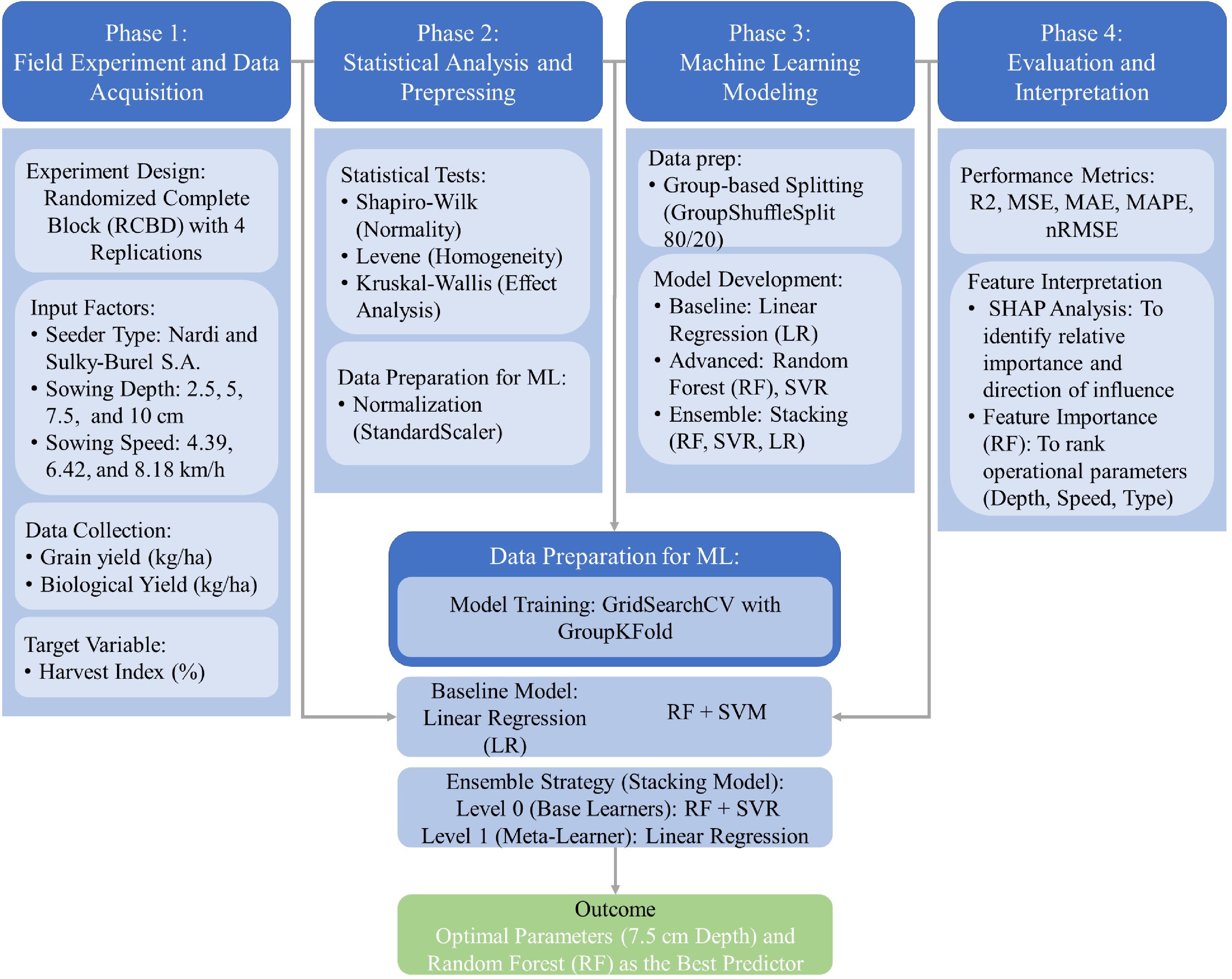
Figure 1. 

Research methodology used.

Experiment site and data collection

The experiment was conducted in a wheat crop field at the College of Agricultural Engineering Sciences, University of Baghdad, Baghdad, Iraq. The study employed a Randomized Complete Block Design (RCBD) with a replication of four. The factors involved were seeder type (Sulky-Burel S.A. and Nardi-TSD), sowing speed (4.39, 6.42, and 8.18 km/h), and sowing depth (2.5, 5, 7.5, and 10 cm). The study registered all seeding factors accurately. Seeding parameters, such as seeder type, sowing speed, and depth settings, were accurately recorded. The two mechanical seeders used are powered by a Massey Ferguson 399 Tractor. The Nardi-TSD Italian seeder is a heavy model with a cutter blade designed for disintegrating soils/soil batterers. The Sulky-Burel S.A. French seeder is lighter. Table 1 below includes their technical and engineering details of each seeder, while Fig. 2 displays images.

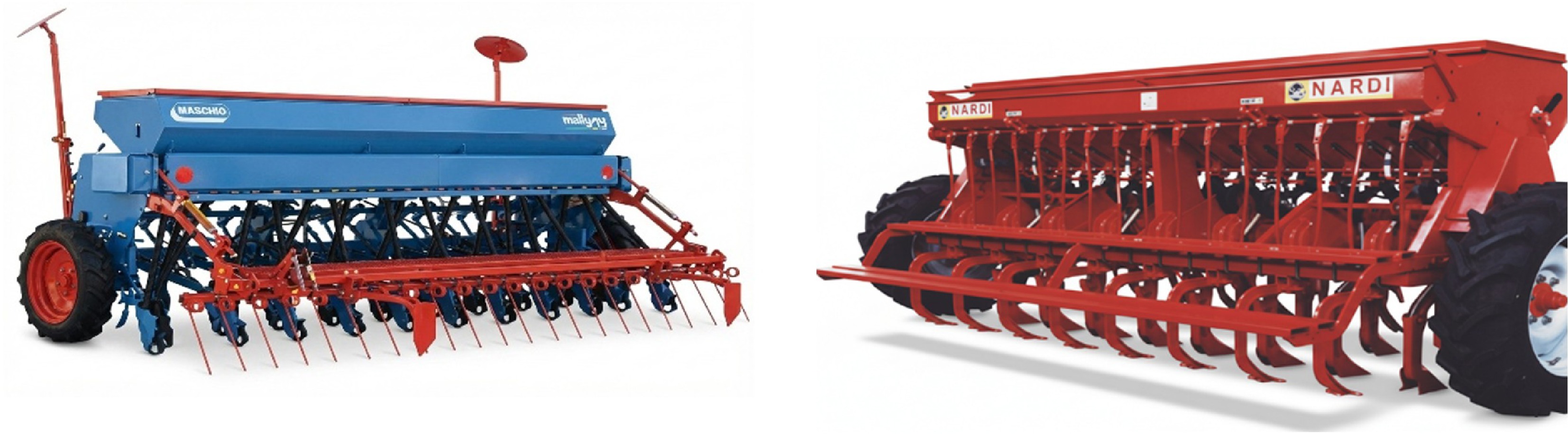
Figure 2. 

Seeders used: (a) Sulky-Burel S.A., and (b) Nardi-TSD.

At physiological maturity, wheat was harvested in specific quarters to measure grain yield and total aboveground biomass. The HI was calculated as the ratio of grain yield to aboveground biomass, as shown in Eq. (1)^[5]:

where GY is grain yield (kg/ha), and BY is biological yield (kg/ha).

Before developing the model, a statistical evaluation of the initial experimental results was performed to assess the distribution and quality of the available data. The Shapiro-Wilk test was used to confirm normality, and the Levene test was used to confirm homogeneity of variances between treatments. Because some data components did not meet the criteria for parametric testing, the Kruskal-Wallis test was used to analyze the significance of both the principal factors and the interactions between the sowing factors to determine the HI. To determine specific differences between groups and identify the optimal levels, Dunn's post hoc test with Bonferroni correction was subsequently applied for pairwise comparisons. To overcome the limitations of single tests in revealing interrelationships, the Generalized Linear Model (GZLM) was used. This model enabled the analysis of interaction effects between seeder type, sowing depth, and sowing speed, providing a deeper understanding of how these parameters interact and their combined effect on the wheat HI.

Data processing and algorithms used

The database included input variables: seeder type, sowing depth measured in cm, and sowing speed measured in km/h. The target variable was the HI measured as a percentage. Ninety-six samples were employed (comprising 24 treatment combinations with four replicates each). To ensure that there was no data leak during the evaluation of the models on unseen treatment conditions, a true form of group-based splitting was implemented. First, a unique group identifier was assigned to each of the 24 different experimental treatment combinations. Then, the dataset was split into a training set and a testing set in the ratio of 80:20 using the GroupShuffleSplit method. This approach ensures that all four samples belonging to a particular treatment combination are present together in either the training or the testing set. After splitting the dataset, normalization was done on the features using the StandardScaler method, ensuring that there was no leak of information from the test set to the training set. This splitting ensures that the training set acts as a strong learning platform, while the test set acts as a genuine test to evaluate the model's learning capability on unseen seeder configurations.

Following this rigorous group-based data split, the features underwent an intensive preprocessing phase to ensure optimal algorithm performance and data compatibility. More importantly, in order to completely eliminate any possibility of data leakage, the parameters used in any scaling and encoding were derived only from the training subset and subsequently applied to the testing subset. First and foremost, the features were distinguished between numerical and categorical features. In this regard, numerical features such as sowing depth and sowing speed were processed using the StandardScaler method. This approach ensures that the features are normalized, and that no single feature dominates the learning process due to its magnitude. This is particularly vital when using distance-based algorithms such as SVR. On the other hand, categorical features such as seeder type were processed using the OneHotEncoder method. This ensures that no ordinal relationships are forced between any two features.

Several regression models were developed, with linear regression being the baseline reference model. To tackle the complex and non-linear nature of the data in the agricultural field, more sophisticated machine learning approaches were utilized and comparatively evaluated; namely, RF, SVR, and a stacking ensemble model. The rationale behind the utilization of the stacking ensemble model is based on the assumption that the diverse range of learning approaches might enable the model to more accurately identify the underlying distribution of the data with respect to various operational parameters of the seeder. RF and SVR were strategically selected as the base learners in the stacking model owing to their algorithmic diversity. RF is a tree-based bagging model that is naturally robust to outliers and highly effective in identifying complex and non-linear relationships without overfitting the data. Conversely, the SVR is a kernel-based algorithm that is robust to noise and effective for small- and medium-sized datasets. The application of these two distinctive techniques in a stacking framework aimed to embrace a wider range of data pattern spectrums. In this stacking framework, a linear regression model was used as a meta-learner. Rather than using a simple linear combination of results, this meta-learner used ordinary least squares to assign optimal weights to predictions generated by both the RF and SVR models in such a way that overall errors were minimized (Fig. 3). This stacking model was extensively tested against individual performances of both the RF and SVR models to objectively measure which model is more generalizable for this specific agronomic dataset.

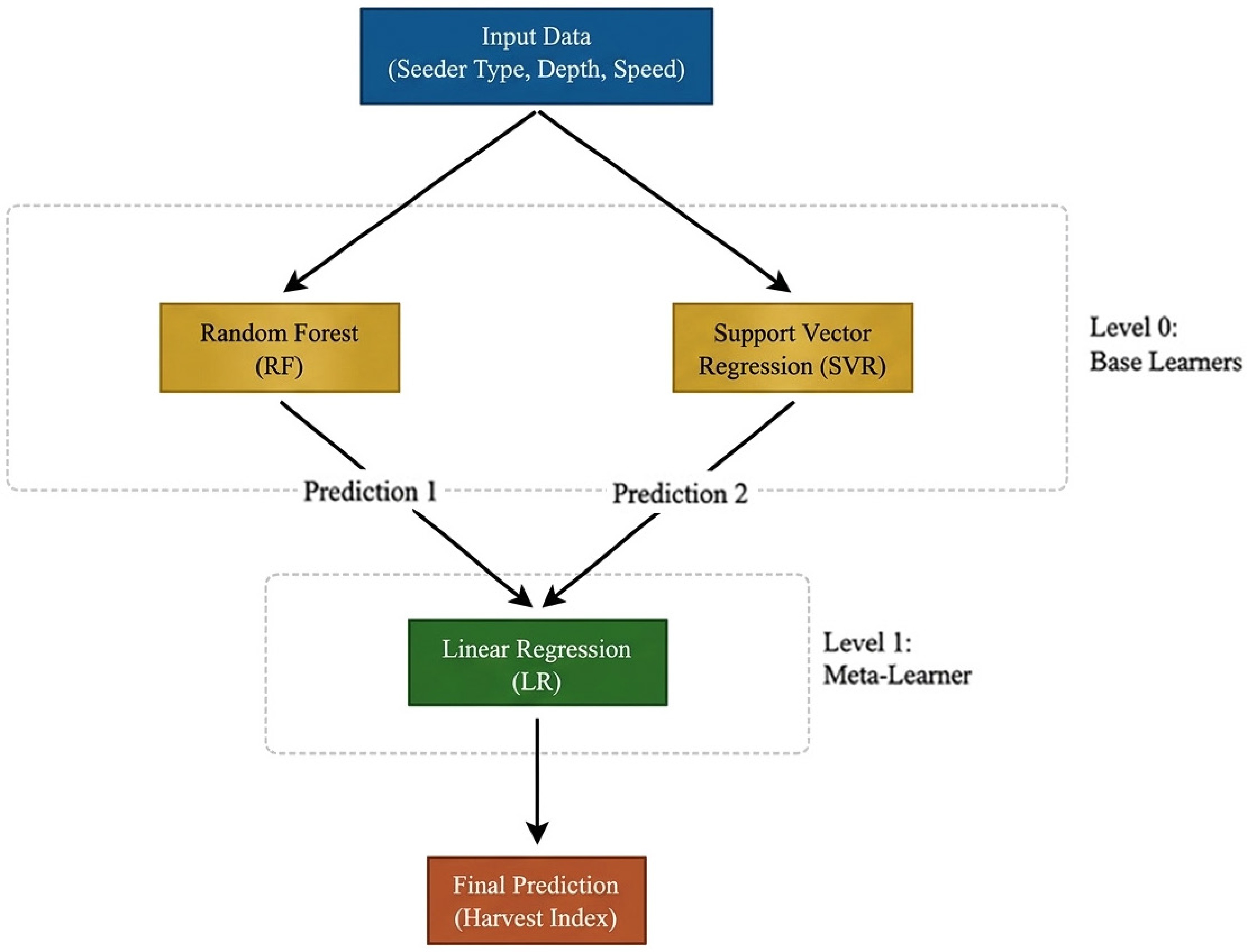
Figure 3. 

Compound stacking model.

All models were implemented using Python 3.x and the scikit-learn library in Kaggle environments. In order to make the algorithms reproducible, the random seed was set to a fixed number (random_state = 42) wherever feasible; however, it is essential to highlight the fact that the actual data division was strictly controlled by the unique group IDs (GroupShuffleSplit) rather than random division. In order to systematically search for the best combination of hyperparameters for the respective algorithms, the GridSearchCV module was used. Importantly, in order to ensure the reproducibility of the experimental replicates and prevent data leakages during the hyperparameter search process, the GroupKFold cross-validation technique was incorporated into the GridSearchCV algorithm, replacing the conventional k-fold cross-validation approach. The expanded hyperparameter search space and the best combination of hyperparameters for the respective algorithms are described in Table 2.

In the context of the stacked ensemble framework under evaluation, the term final estimator corresponds to the meta-learner, which in this case corresponds to the linear regression model. Rather than averaging the predictions made by the base learners (RF and SVR) in a static or simple fashion, the meta-learner uses a dynamic approach. The predictions made by the base learners on the data instances in the folds are provided as input to the meta-learner, which in turn uses the ordinary least squares problem to find the optimal coefficients for the input provided by the base learners in order to minimize the training error.

In addition, to ensure that the models are reliable and accurate, a series of accurate results were calculated for predictive performance in the process of both training and testing, which included nRMSE, MAE, R², MSE, and MAPE. To standardize the variable annotations in the above formulas, let w_t denote actual (measured) values, and w_f denote forecasted (predicted) values by the model for a total of N data points. Moreover, let w_tmax and $ \mathrm{w}_{\mathrm{t}}^{-} $ denote the maximum and mean of actual values, respectively. The above metrics were computed according to Eqs (2)–(6)^[25,26]. At the same time, other experiments, such as correlation analysis and feature importance analysis were conducted to examine which factors were most impactful in differentiating the values of the HI.

where, w_f, w_t, and w_tmax represent the forecasted values at each time point, the observed/measured values at each time point, and the maximum observed values, respectively. $ w_{t}^{-} $ refers to the arithmetic mean of the actual (true) values. N is the number of data samples for the time scale.

Field data were analyzed to examine the effect of the studied variables, including seeder type, sowing depth, and sowing speed, on the HI, with a focus on intra-sample variance and the suitability of the data for the applied statistical analysis. Table 3 illustrates the statistical analysis and the non-parametric variance test.

The test statistic for the normality test in the case of the HI is presented in Table 3. The test revealed that the HI does not fulfill the assumption of normality for several treatments. The Shapiro-Wilk test was significant (p < 0.05) for the sowing depth of 7.5 cm (p = 0.03) as well as the sowing speed of 8.18 km/h (p = 0.004) for the two kinds of seeder. The Levene's test was also significant, indicating the presence of unequal variances in the groups for sowing depth, sowing speed, and the two kinds of seeder. The implication was that the study variables are not normally distributed, meaning that the application of parametric tests was inappropriate. The Kruskal-Wallis test was used to test the groups for the non-parametric test. Analysis using the Kruskal-Wallis test revealed that the factor of sowing depth has a highly significant effect on the HI (p < 0.01; H = 78.53). This result verified that the variance of the HI is greatly related to the sowing depth of the seeds. This result is not uncommon, as various studies have revealed the significance of planting depth towards germination and growth. For instance, Larsson^[13] demonstrated that the difference in the sowing depth greatly impacts the growth parameters and yield of wheat. However, there were no statistically significant differences in seeder type (H = 1.12, p = 0.28), which corresponds to the opinions of Bhatti et al.^[9], who believe that seeder type differences may be less substantial compared to depth and speed. In relation to the speed of sowing, with an H-statistic of 0.74 and a probability of 0.68, it is clear that differences in speed were not statistically significant in this study, so it is also possibly less sensitive or may require further study in relation to other variables^[10]. Consequently, the findings from these results clearly show that the most determining factor for the HI is the sowing depth, whereas the seeder type and the sowing speed were found to be insignificant within the given scope.

Although the Kruskal-Wallis test identified the single major factor of sowing depth, it is not sufficient to show the relationships that exist between various factors. As a result of the need to understand the intricate relationships that exist between the various seeding parameters, advanced statistical analysis was carried out, and the results of the GZLM are shown in Table 4.

The results demonstrated by Table 4 show the intricate but highly significant interactions between the parameters included in the study. First and foremost, the combination of seeder type and sowing depth has demonstrated a statistically significant effect on the results, with the p-value being 0.00. This implies that the effect of the HI on the depth is not fixed but depends on the design characteristics of the seeder. Furthermore, the interaction between the examined parameters, that is, the combination of depth and speed is also highly significant, as their respective p-values are 0.00. This implies the degree of sensitivity that the mechanism has to the correct functioning of the sowing depths, regardless of the speed applied. Perhaps the most important result, however, is the demonstration of the significance of the three-way interaction between the examined factors, as their combined result has a p-value of 0.00. On the other hand, the combination of seeder type and sowing speed does not manifest itself as being significant, as the p-value is 0.21.

Having demonstrated a statistical significance for sowing depth but a lack thereof for the remaining variables from Table 3, we now turn to a graphical exploration of how the HI is affected by such variables. Figure 4 has been structured with a, b, and c sections, with the purpose of providing a proper characterization of the trends that are available within the variables, and how they are spread around, with consideration of their significance on their own merits.

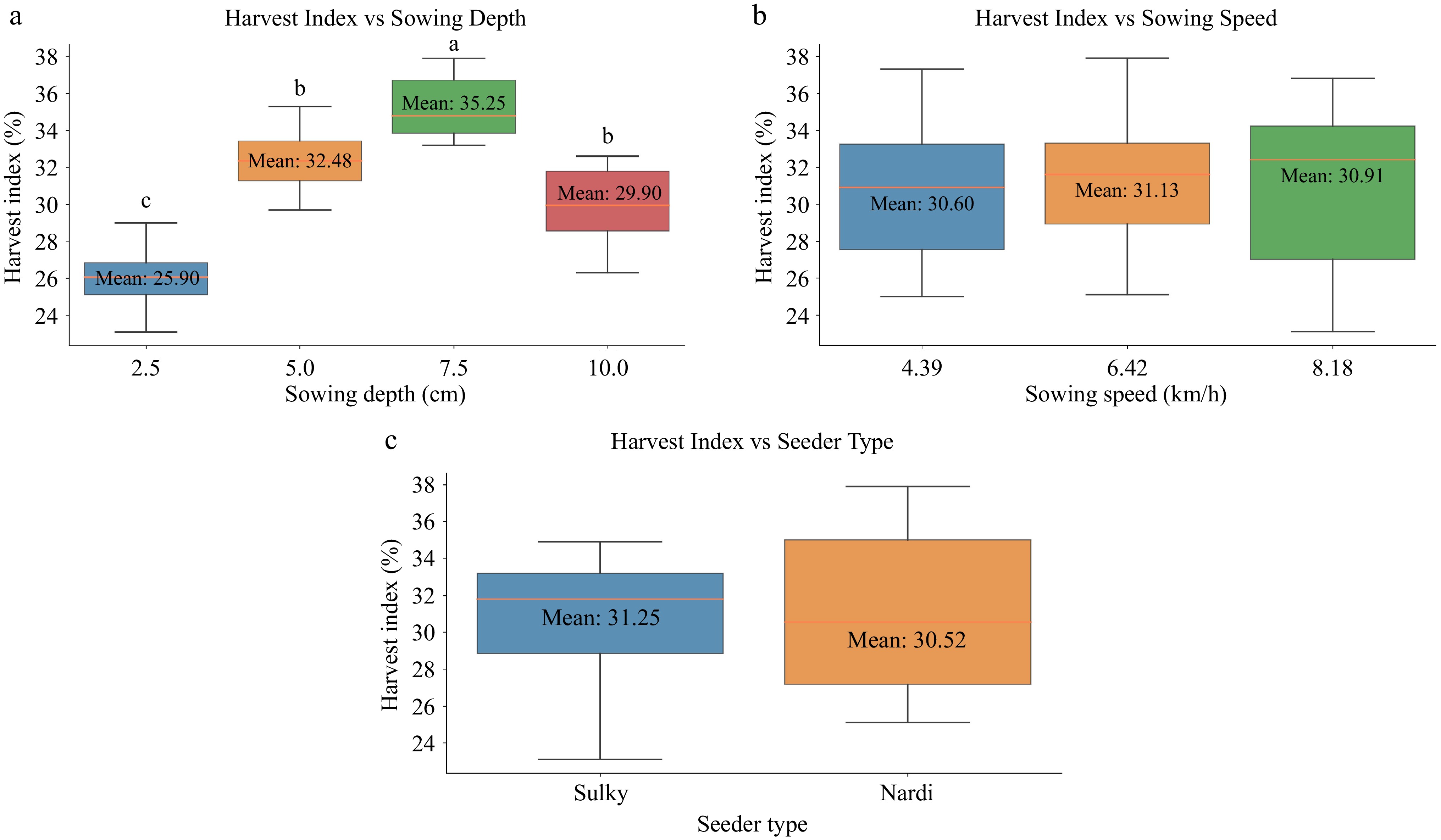
Figure 4. 

Effect of basic operating parameters on HI: (a) seeder type, (b) sowing depth, and (c) sowing speed.

Turning to Fig. 4, specifically 4a, a comparison between the Sulky and Nardi HI indicate they are quite similar, since the Sulky HI is 31.25% while Nardi HI is 30.52%. Nardi HI varies a bit more. The convergence of the HI means that both seeders achieved a similar longitudinal distribution, which reduced competition between plants for light and nutrients. The type of seeder appears not to make any difference to HI in this scenario because there is no distinguishable difference in their performance. In Fig. 4b, there is an examination of how HI varies depending on the level of sowing depth. The values above average relate to an HI of approximately 35.25%, which occurs at a depth of 7.5 cm, as opposed to 2.5 and 10 cm, which record low harvest indices of approximately 25.90 and 29.90%, respectively. There appears to be a need to identify the accurate depth that has a positive impact on harvest productivity. Dunn's post hoc test with Bonferroni correction shows that the results revealed that the HI at 7.5 cm was significantly higher (p < 0.05) than all other depths (2.5, 5, and 10 cm), while no significant difference was found between 5 cm and 10 cm (p > 0.05). This confirms that 7.5 cm is the statistically confirmed optimal depth for maximizing HI. The 7.5 cm sowing depth can function best since it offers a stable hydrothermal condition. This middle ground would provide access to constant moisture in the soil without additional energy expenditure, which would be experienced in deeper planting (10 cm), while it would also avoid drying and the formation of a crown roots with shallower planting (2.5 cm)^[27]. Figure 4c examines the sowing speed. The average HI of corresponding sowing speeds of 4.39, 6.42, and 8.18 km/h is closely grouped around the average HI, ranging approximately between 30.60 and 30.91 km/h. This makes the HI insensitive to the sowing speed. The stability of the harvest indicator at different speeds indicates that the seeder was stable during sowing; thus maintaining a stable depth even with increased speed, which prevented crop deterioration. To sum up, these data indicate that sowing depth is the most important factor to improve HI, and optimum sowing depth can improve the efficiency of harvest. The factors of seeder type and sowing speed do not have a great influence on HI. Although the individual effects of both seeder type and sowing speed appeared limited when studied independently in Fig. 4, GZLM analysis demonstrated that their true value emerges from their interaction with sowing depth.

For the purpose of determining the strength of the correlation between inputs, including operating factors, and the HI, Fig. 5 shows the results of the SHAP (SHAP Summary Plot) analysis, which reveal the relative importance and direction of influence of each of the study factors on the prediction of the HI.

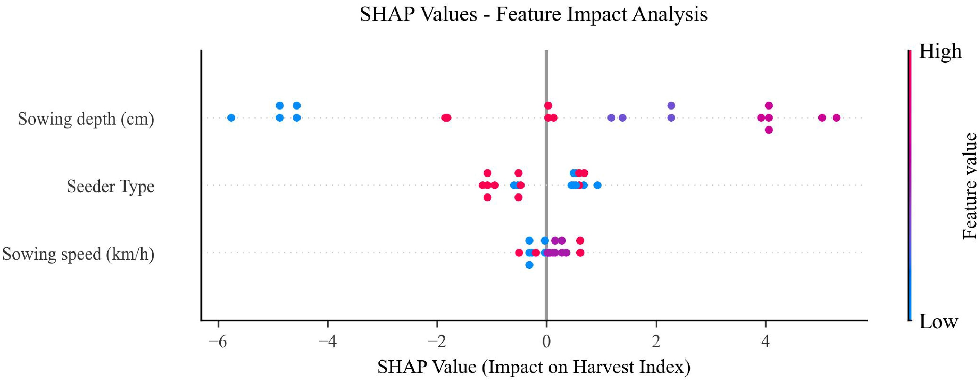
Figure 5. 

SHAP diagram showing the relative importance and direction of influence of operators on the prediction of the HI.

In the SHAP values plot, it's clear that the depth of sowing is the most important factor in the system, more important than all other mechanical factors combined. The scattering of values on the plot reveals a positive relationship between depth and HI when sowing depth is increased. The practical meaning of this mechanical discovery is that the 7.5 cm depth treatment performed remarkably because it produced a perfect root development environment that led to high harvests. Contrary to the previous result, the values for the speed of sowing and seeder type are close to zero and have a small range, meaning they have a small contribution to the accuracy of predictions regarding depth. This result matches the statistical test, where there were no differences between the mechanical factors regarding depth, giving more flexibility to the grower to choose the speed and seeder type without affecting HI.

Having identified the parameters influencing HI and understood their respective impacts on it via SHAP analysis, it was time to subject these models to a quantitative test to evaluate their appropriateness and accuracy. The intention was to validate these models and test them against a basic linear regression model to see if they could compete with RF-SVR models and a stacking model. In addition to these tests to provide generalizability and avoid over-modeling bias, all models were subjected to train and test evaluation metrics, including accuracy and error measurement described in Table 5.

The results obtained in Table 5 indicate a significant disparity in the predictive ability of the considered algorithms. It has been observed that the sophisticated machine learning algorithms, specifically the RF algorithm, performed significantly better than the conventional baseline predictive model, which was based on the linear regression technique, in terms of all the accuracy and error-related measures (R², MSE, MAE, nRMSE, MAPE). It has also been observed that the RF model was the best in achieving the highest level of predictive accuracy in the rigorous testing phase, where new groups were considered (R² = 75.08%). Although it was expected that there would be a drop in the accuracy level in the testing phase, as compared to the training phase, due to the elimination of the data leakage aspect, the RF model was the best in achieving the highest robustness in the prediction task. Furthermore, it has also been observed that the stacking and SVR-based models performed moderately well in the prediction task, but were still better than the conventional linear regression-based predictive model, which performed poorly in capturing the variability in the data set (R² = 62.2%). This again underlines the limitations of using simple linear techniques to address complex non-linear relationships between various operational aspects of the seeder and HI, thereby reiterating the need for using robust AI techniques such as RF for making precise agricultural predictions.

Although the stacking model's accuracy is good, it is important to peek under the hood and to see which physical variables drive its predictions. To do this and make sense of the numbers in practical farming terms, the RF approach was implemented and used to pull out 'Feature Importance Scores'. This works well because it essentially measures how much model performance decreases as each variable is turned off. The aim here is to rank the seeder parameters (type, depth, and speed) by the impact on the HI value. Figure 6 depicts the results of this analysis.

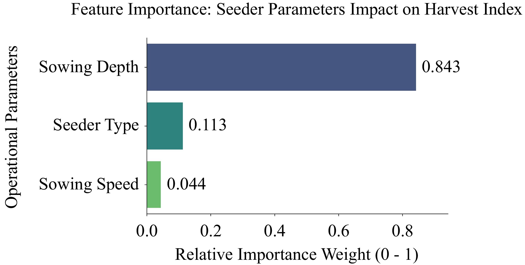
Figure 6. 

Feature importance: seeder parameters' impact on HI.

Figure 6 presents the ranking of the different operational variables in terms of their importance, as derived from the RF model. It is evident that sowing depth dominates because it is the most influential factor for the HI prediction, taking up the largest share of the model's effect. This agrees perfectly with our statistical findings and reinforces the model in terms of capturing the true causal relationships. It also makes physiological sense because depth directly shapes the germination environment and root development. On the other hand, the seeder type and sowing speed are of minor importance compared to depth, which is in good agreement with the statistical conclusion that these two factors do not differ very much in their effect. This consideration has practical and engineering implications: what really matters is to get the right sowing depth, whereas the choice of the seeder is less important. Furthermore, increases in sowing speed aimed at enhancing field capacity may be acceptable and thus not harmful to productivity, provided the depth remains constant.

Despite the limitations imposed by the size of the dataset collected from field trials, the implementation of a rigorous group-based cross-validation strategy has proved to be highly effective in preventing data leakage and providing a realistic evaluation of the models. This has clearly demonstrated that advanced machine learning algorithms, in particular RF, can be effectively implemented in agricultural settings, where it is sometimes challenging to compile massive datasets. From an agronomical perspective, this research has provided valid and insightful information regarding the complex inter-relationships between seeder operating factors and wheat HI. Even though sowing depth has proved to be an important factor, it is essential to model all the variables in an exhaustive manner to enhance precision farming. The accuracy of the RF model has ensured its effectiveness in providing precise predictions for completely unseen seeder configurations. The findings from this research clearly demonstrate the immense potential for effectively utilizing rigorously validated AI and ML for sustainable resource management and adapting to the dynamic complexities in modern agriculture.

Through this combination of field experimentation and advanced ML modeling, this research has been able to conclusively establish that sowing depth is the most critical operational factor that impacts wheat HI, with 7.5 cm being established as the optimal depth. On the other hand, it has also been concluded that seeder type and sowing speed were not critical limiting factors. This is important because it ensures that wheat farmers have the operational flexibility to increase sowing speeds. In terms of predictive modeling, this study has also been able to conclusively establish that traditional statistical modeling techniques, such as linear regression possess limited potential to capture the complex relationships that are characteristic of agricultural data. On the other hand, this study has been able to conclusively establish that AI modeling techniques possess vastly superior predictive modeling potential. In this respect, it has been conclusively established that once a rigorous cross-validation strategy is implemented to totally eliminate any scope for data leakage, the RF model possesses the highest robustness potential and is able to produce a realistic predictive accuracy (R²) of 75.08% on completely unseen wheat sowing configurations. These predictive modeling results were strictly corroborated using SHAP analysis.