Optimized configuration and characterization of LCC-S based wireless power transmission system

Wireless Power Transfer (WPT) technology is garnering significant attention as it enables the transmission of electrical energy from one location to another without the need for conventional wire connections. This field is continually advancing, bringing innovation and convenience to various domains. With the proliferation of electronic devices such as mobile devices, electric vehicles, and wearable technology, the demand for WPT technology is steadily increasing due to its ability to provide a more convenient method of charging. In comparison to traditional wired methods of electrical energy transfer, WPT technology overcomes several limitations, including the constraints of charging cables, contact resistance losses, and the lack of portability associated with cables. Hence, it holds vast prospects for numerous applications^[1−5].

In recent years, Magnetic Coupling Resonant Wireless Power Transfer (MCR-WPT) systems have garnered significant research attention due to their advantages in high power and efficiency^[6,7]. In this system, to enhance transmission performance, both primary and secondary sides require the use of compensation networks. The selection of compensation network topology and optimal parameter configuration can impact the system's operational characteristics, as well as the voltage and current loads on components. To address the detailed design issues of ICPT (Inductive Coupling Power Transfer) systems, researchers utilized an optimization algorithm applied to the battery charger of ICPT. They also introduced a new design factor, KD, to select the optimal configuration among four basic topologies^[8]. To enhance transmission efficiency, researchers optimized the PS-type ICPT system using a genetic algorithm, but they did not achieve the simultaneous maximization of both transmission efficiency and power^[9]. Considering the proximity effect and skin effect of the transmitter and receiver coils, researchers introduced an adaptive weight-adjusted particle swarm optimization algorithm to optimize the S-S topology^[10]. Compared to traditional SS, SP, PS, and PP compensation topologies, the LCC compensation network offers many apparent advantages^[11,12]. By adjusting the parameter configuration and operating frequency of the compensation network^[13], constant voltage or constant current characteristics can be achieved, allowing for easy implementation of Zero Voltage Switching (ZVS)^[14], and reducing switch losses^[15−19]. Therefore, LCC compensation networks have received significant attention in the field of electric vehicle charging. Researchers proposed a genetic algorithm-based optimization method for LCC-S system parameters to achieve constant current or constant voltage output characteristics in various operating modes, without specific restrictions on the output power range^[20].

The 'frequency splitting' phenomenon is typically caused by strong magnetic coupling within the system. The interaction between resonators can lead to a deviation of the system's operating frequency from its inherent resonant frequency, thereby affecting transmission efficiency and power output. This phenomenon becomes more pronounced when the coupling coefficient is high, as increased coupling strength can induce multiple resonant frequencies, causing the operating frequency to deviate from the initially designed resonant frequency. To enhance the system's transmission efficiency and power output, this paper optimizes the ratio between the operating frequency and the resonant frequency. Additionally, the inductance ratio between L_f and L_l also has a significant impact on system performance, and thus, this paper also addresses its optimization. This paper presents an improved particle swarm optimization algorithm that uses chaotic mapping to initialize the particle population and updates the positions of the particles with improved Lévy flights and achieve maximum efficiency under constraints.

The equivalent circuit of the LCC-S magnetically coupled resonant wireless power transfer system is shown in Fig. 1.

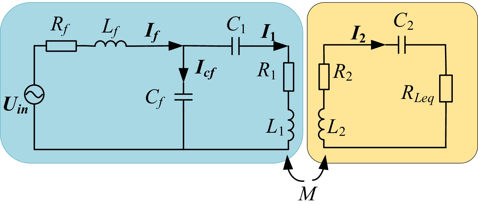
Figure 1. 

Equivalent circuit of the LCC-S WPT system.

In Fig. 1, U_in represents the output voltage after inversion, L_f is the compensating inductance on the transmitter side, L₁ and L₂ are the inductances of the transmitter and receiver resonant coils, C_f is the parallel compensating capacitance on the transmitter side, C₁ and C₂ are the series compensating capacitances on the transmitter and receiver sides, I_f denotes the output current after inversion, I₁ and I₂ are the resonant currents on the transmitter and receiver sides, respectively. R_f represents the parasitic internal resistance of the compensating inductance on the transmitter side, while R₁ and R₂ are the parasitic internal resistances of the resonant coils on the transmitter and receiver sides, respectively. R_Leq is the equivalent load resistance.

Mathematical model

For ease of calculation, the receiver-side circuit is mapped to the transmitter side, resulting in the equivalent circuit shown in Fig. 2.

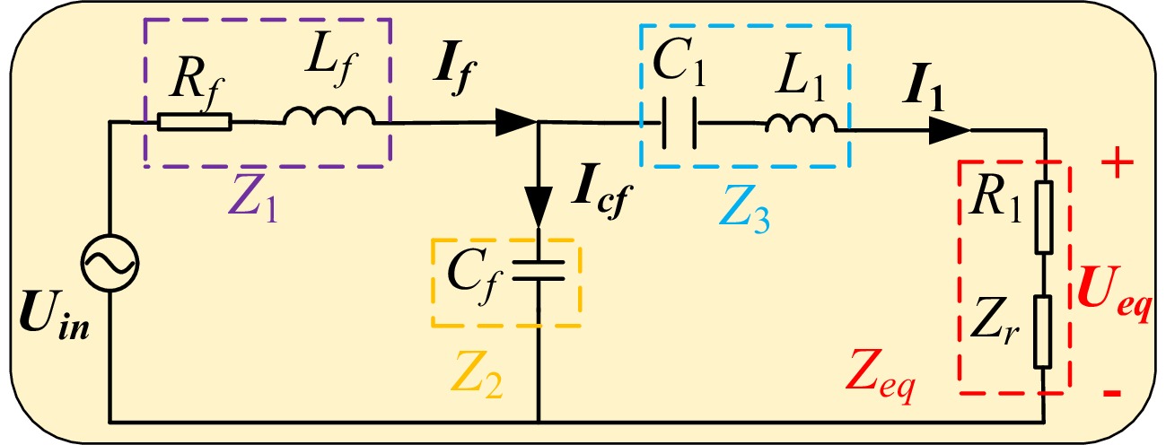
Figure 2. 

LCC-S primary side equivalent circuit.

The resistance impedance of the receiving circuit is:

The equivalent reflection resistance to the transmitter side is:

Using the two-port theory to establish a mathematical model and derive it:

where, A₁₁, A₁₂, A₂₁, and A₂₂ are two-port A parameters. U_eq is the sum of the voltages of the reflected impedance Z_r and the internal resistance R₁ of the transmitting coil.

To provide a better description, one can choose to replace the original topology structure with a T-network for compensation:

where, P = Z₁Z₂ + Z₂Z₃ + Z₁Z₃, Z₁ = R_f + jωL_f, $ {Z_2} = \dfrac{1}{{j\omega {C_f}}} $, and $ {Z_3} = j\omega {L_1} + \dfrac{1}{{j\omega {C_1}}} $.

From this, the input impedance of the system can be calculated:

Referring to Eqn (3), it is possible to calculate the inverter output current, transmitter coil, and receiver coil currents:

The expressions for input and output power can be derived as follows:

where, $ {R_{Leq}} = \dfrac{{8{R_L}}}{{{\pi ^2}}} $, R_Leq is the rectifier circuit and load-side equivalent resistance.

With reference to Eqns (9) and (10), the transmission efficiency can be obtained as:

To enhance the transmission performance of the system, the transmission efficiency of the system is set as the optimization objective function, and an improved particle swarm algorithm is employed to optimize the relevant parameters.

Transmission performance analysis of the system

This paper is based on the mathematical model of a wireless power transfer system with an LCC-S topology. The study delves into the transmission characteristics of the system in terms of the operating frequency, transmission side compensation inductance, and load impedance. When investigating the transmission characteristics of the system, it is necessary to establish clear relationships between the parameters, which are configured as follows:

where, n is the ratio of the transmitter-side compensation inductance to the transmitter-side resonant coil inductance and ω_n is the ratio between the transmitter-side compensation inductance and the transmitter-side resonant coil inductance. ω₀ is the intrinsic resonant angular frequency formed by the compensation network and the coil, where ω₀ = 2πf₀ and f₀ is the resonant frequency of the system. ω represents the operating angular frequency of the system, where ω = 2πf and f is the operating frequency of the system.

Based on the QI wireless charging standard, the initial parameters of the LCC-S wireless power transfer system in the magnetic coupling resonance (MCR) mode are determined, as shown in Table 1.

Figure 3 illustrates the impact of varying operating frequencies on the system's transmission efficiency and output power. When the system's operating frequency is close to the resonance frequency point, the system operates in a fully resonant state, resulting in minimal losses and the highest transmission efficiency. However, the output power reaches its peak value at the resonance frequency point but does not reach its maximum value. Therefore, when optimizing the system's operating frequency parameter configuration, it is essential to strike a balance between transmission efficiency and transmission power to meet the desired objectives.

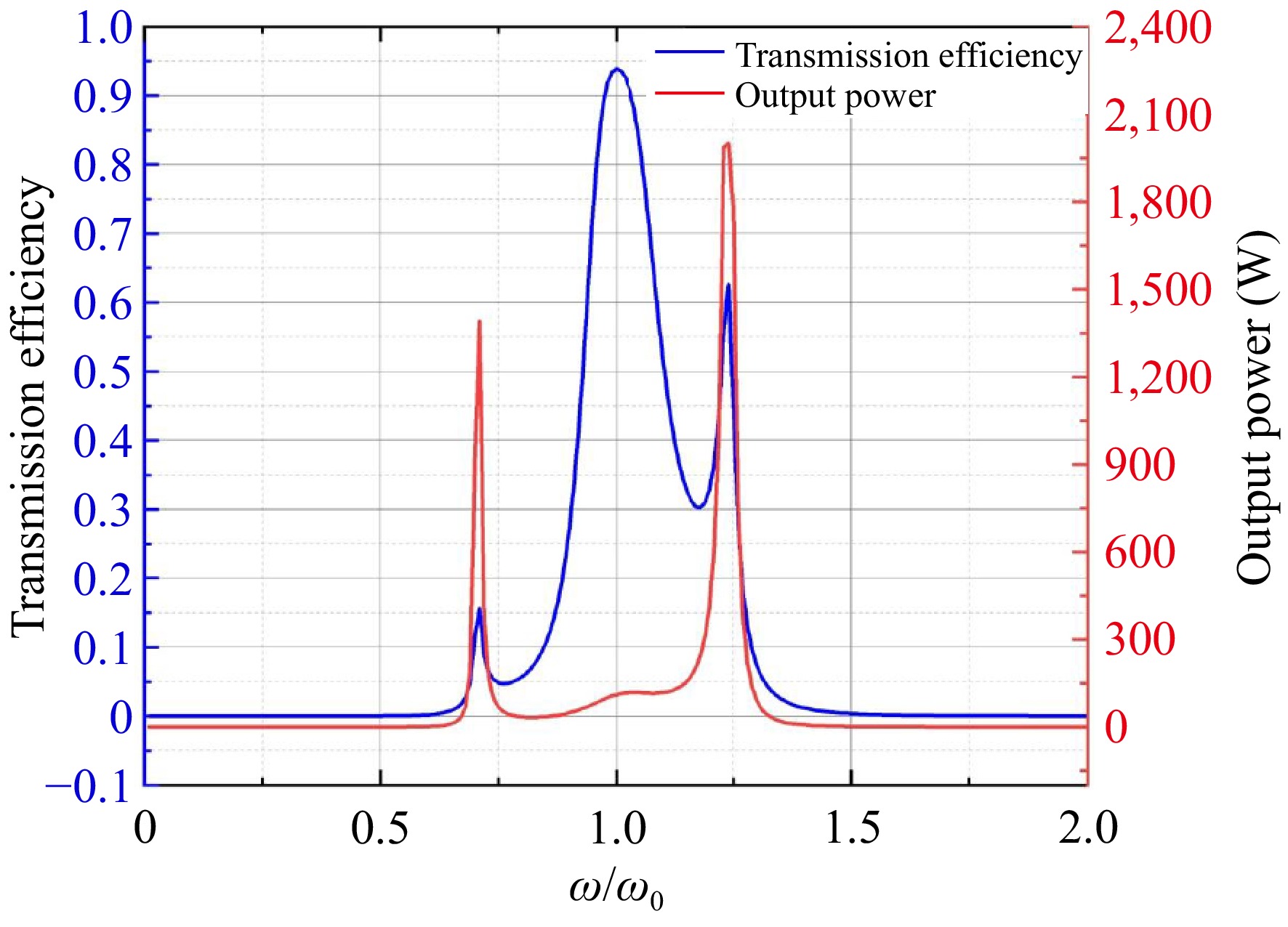
Figure 3. 

Curves of operating frequency and transmission characteristics.

Figure 4 illustrates the simulation results analyzing the impact of changes in L_f/L₁ on the system's transmission performance, based on the initial parameters listed in Table 1. The study specifically investigates how the compensation inductance influences the transmission characteristics of the system, particularly within an LCC topology network. The ratio L_f/L₁ is used as an optimization variable to maximize the power and transmission efficiency of the wireless charging system. The correct ratio can reduce losses within the system, ensuring more efficient energy transfer. As shown in Fig. 4, when the ratio is close to 1, the efficiency is high but nearly constant, while the power becomes very small. Therefore, L_f is set to nL₁, with n typically ranging between 0 and 1. To ensure that the system operates stably and maintains resonance at an operating frequency, it is necessary to synchronously adjust the values of the compensation inductor L_f and the capacitors C_f and C₁. Figure 4 demonstrates the correlation between the output power of the system and the transmission efficiency when the compensation inductance is varied. It can be observed from Fig. 4 that the transmission efficiency of the system initially increases rapidly when the compensation inductance is increased, but when a certain threshold is reached, the increase in transmission efficiency becomes relatively slow. On the other hand, when the output power is increased up to a certain critical value, it decreases sharply, which indicates that there is a maximum output power value in the system. Therefore, the value of the compensation inductor must be optimally configured during parameter design to meet the transmission performance requirements of the system.

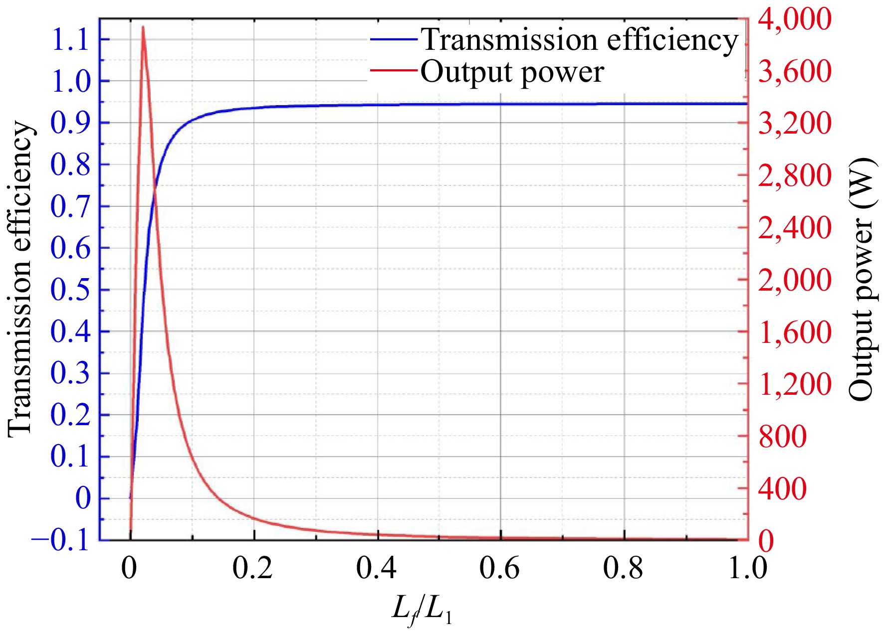
Figure 4. 

Curves of compensating inductance and transmission characteristics.

In real wireless charging application scenarios, the load resistance value usually fluctuates within a certain range because the state of the charging object changes frequently. Assuming that the system operates at resonant frequency, its load resistance varies from 0 to 100, and other simulation parameters are shown in Table 1. Figure 5 shows the relationship between the transmission performance of the system and the load resistance value at 85 kHz. From Fig. 5, it is evident that when the system is in a state of full resonance, the initial transmission efficiency rapidly increases with an increase in load resistance. Once efficiency reaches its peak, the rate of improvement in transmission efficiency begins to slow down. However, in the initial stages, the output power instantly reaches its peak, and as the load resistance gradually increases, the system's output power rapidly decreases. This phenomenon is because when the system operates at the resonance frequency, the effect of parasitic parameters is disregarded, and the output can be approximated as a constant voltage source. Consequently, the output power is inversely proportional to the square of the load resistance.

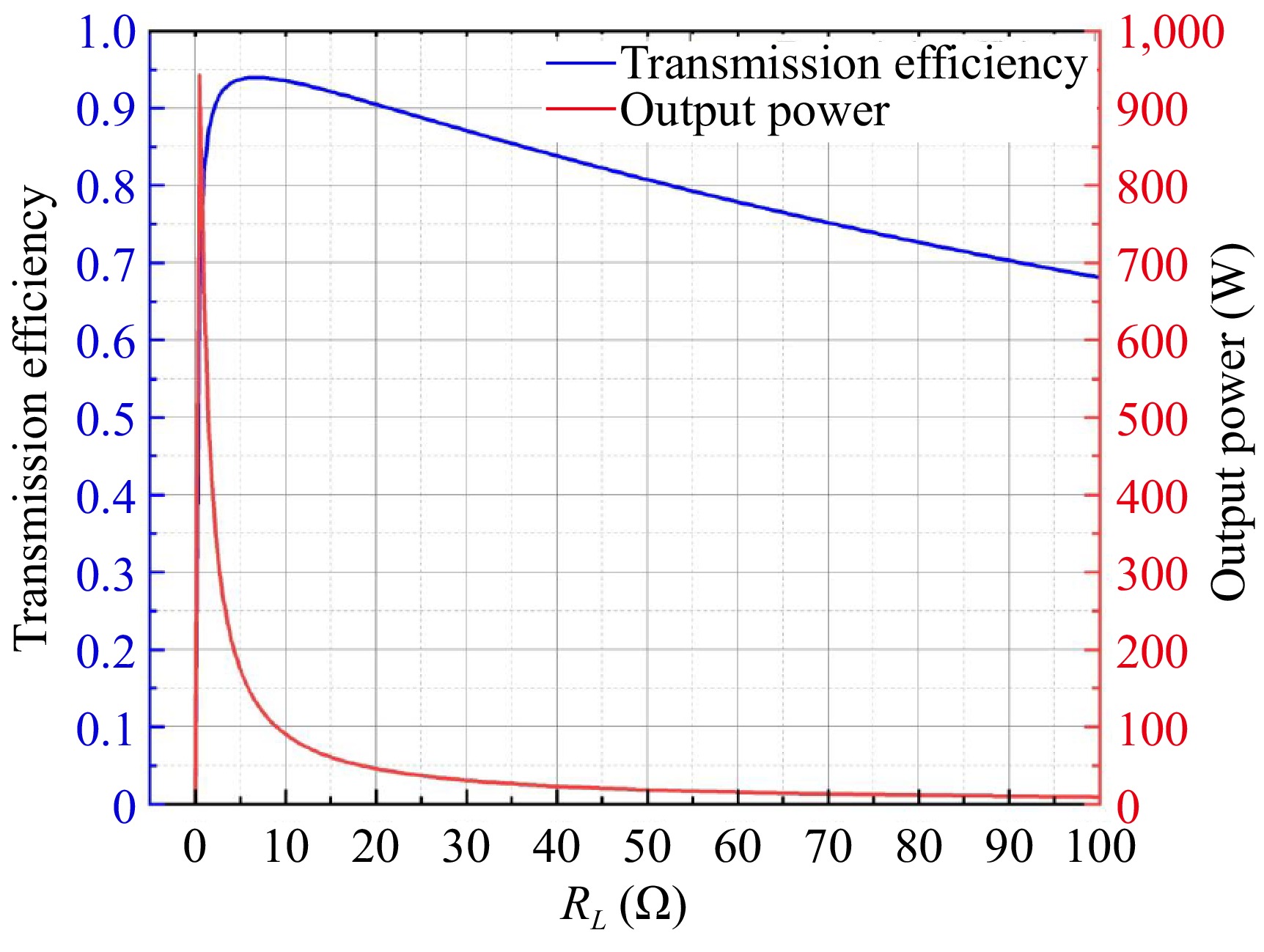
Figure 5. 

Curves of load resistance and transmission characteristics.

Concerning Eqn (12), in wireless power transfer systems, there is a significant correlation among the parameters of the compensation network, which has a substantial impact on the overall system performance. Therefore, when designing the system, it is necessary to consider multiple performance factors such as transmission efficiency, output power, and component stress. In such cases, selecting one performance metric as the optimization objective while considering other performance metrics as constraints is of great significance.

Optimization of the model

The transmission efficiency derived from the mathematical model of the LCC-S wireless power transfer system is used as the optimization objective function:

When studying operating modes within a wide frequency range, the working frequency f is chosen as the first optimization variable. After determining the coupling mechanism, the selection of parameter n directly influences the transmission performance. Therefore, n is utilized as the second optimization variable. Hence, the final set of optimization variables is x = [f, n]^T. Through algorithmic optimization, improved operating frequencies, and compensation network component parameters can be achieved. It is also necessary to consider nonlinear constraints on component voltage stress, current stress, and output power, as referenced in Eqn (14).

where, lb and ub are the lower and upper bounds of the optimization variables respectively, $ {I_{{C_f}}} = \left| {{I_f} - {I_1}} \right| $, $ {C_f} = \dfrac{1}{{{\omega _0}^2{L_f}}} = \dfrac{1}{{{\omega _0}^2n{L_1}}} $, $ {C_1} = \dfrac{1}{{{\omega _0}^2({L_1} - {L_f})}} = \dfrac{1}{{{\omega _0}^2{L_1}(1 - n)}} $.

Traditional PSO algorithm

The traditional particle swarm algorithm originates from simulating the principles of collective behavior in biological populations, especially cooperative foraging. This bio-inspired algorithm has found extensive application in the field of highly efficient parallel optimization. The particle swarm algorithm, by simulating cooperative behavior among particles, continuously searches for the optimal solution in the solution space through iterative processes to address highly nonlinear and high-order optimization problems. Compared to genetic algorithms, the particle swarm algorithm boasts numerous advantages, including faster execution, reduced computational burden, and fewer tunable parameters^[21]. In the particle swarm algorithm, a group of particles is initially randomly distributed in the optimization space. During each round of the optimization iteration, each particle calculates its distance from the current best solution, which is considered as the particle's fitness with respect to the objective function. The process of updating particle velocity and position is as follows:

where, t represents the iteration number, while v_ij and x_ij represent the velocity and position of the i-th particle, respectively. The historical best solution for the i-th particle is denoted as p_i, and the current global best solution is represented as g_i, c₁, and c₂ represent the inertia weight, local factor, and global factor, respectively. Depending on the specific problem, these parameters can be adjusted appropriately. Setting these parameters correctly is crucial to ensure that the algorithm effectively converges to the global optimum.

The traditional PSO algorithm is prone to getting stuck in a local optimum when dealing with the optimal parameter configuration problem of LCC-S-type systems.

Improved PSO algorithm

To address this issue, this paper introduces a particle optimization algorithm based on improved Lévy flights and chaotic mapping. This algorithm incorporates chaotic mapping for initialization, enhancing the diversity of individual particles over the traditional random initialization. Additionally, it integrates an improved Lévy flight mechanism into the position update formula, which improves search accuracy and aids individual particles in escaping local optima.

(1) Chaos Initialization: In a globally convergent particle swarm optimization algorithm, selecting an appropriate initial population is a critical factor that determines the convergence characteristics of the algorithm. During the initial search process, since the specific location of the optimal solution cannot be determined, the spatial characteristics of the solution can only be described through the distribution of the initial population. When the initial population is selected correctly, after multiple iterations, the algorithm can quickly find the global optimum. To address the population initialization issue, this paper proposes an algorithm combined with chaotic mapping (Logistic).

From Fig. 6, it can be observed that the initial population distribution generated by the chaotic mapping (Logistic) is uniform. The fitness values of random numbers generated by the chaotic mapping are significantly improved. Using chaotic mapping instead of the traditional uniform distribution (rand) random number generator can yield better results, especially when there are many local optima in the search space, making it easier to search for the global optimum.

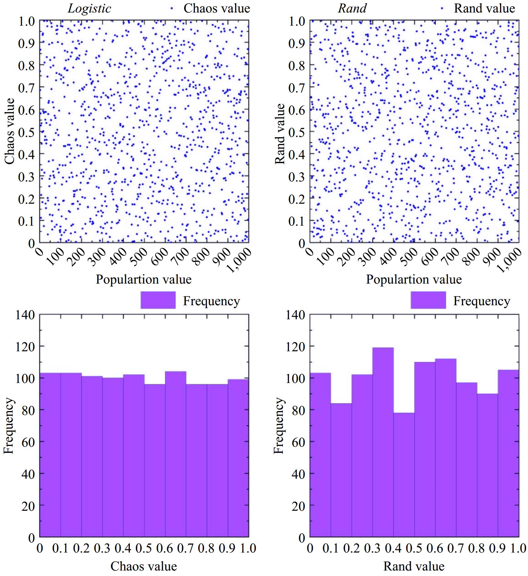
Figure 6. 

Visual comparison of chaotic mapping and stochastics.

(2) Improved Lévy flight: Extensive research has shown that Lévy flight can enhance search efficiency in unstable environments. To validate the superiority of Lévy flight, a graph was plotted in MATLAB to compare the differences between Lévy flight and random walk. From Fig. 7, it is evident that when Lévy flight and random walk have the same number of steps, Lévy flight exhibits stronger search capabilities, thereby expanding the search range. By incorporating it into the particle swarm optimization algorithm, not only can the vitality and leaping ability of the particle swarm be enhanced, but the overall optimization performance of the algorithm can also be improved.

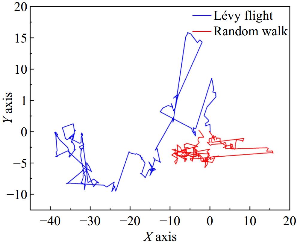
Figure 7. 

Comparison of Lévy flight and random walk.

In this paper, Lévy flight is not directly added to particle updates as in other articles. Instead, it has been slightly modified, and the results are indeed better than directly adding the Lévy coefficient. The principle formula is as follows:

where, α is the step scaling factor and Lévy(β) is the Lévy random path.

where, u denotes the lateral motion, and v denotes the vertical motion.

The principle of the improvement is as follows:

where, α = 0.01, $ \lambda = {e^{\frac{{1 - T}}{{T + 1 - t}}}} $, $ C{\text{ = }}2r(1 - \dfrac{1}{N}) $, r is the number of random free numbers and N is the number of iterations.

The purpose of doing this is to complement the advantages of the particle swarm algorithm with Lévy flight, allowing for the dynamic adjustment of the scale factor for each optimization search.

This section will establish a simulation model under the ChaosLPSO algorithm in MATLAB/Simulink. The first part is simulated in MATLAB, and the second part involves building an LCC-S simulation platform in Simulink to perform simulations for verifying the theoretical analysis mentioned above.

ChaosLPSO simulation

In both the PSO and ChaosLPSO algorithms, the population size is set to N = 5, and the number of iterations is D = 100. The fitness (transmission efficiency) curves for the PSO and ChaosLPSO algorithms are shown in Fig. 8.

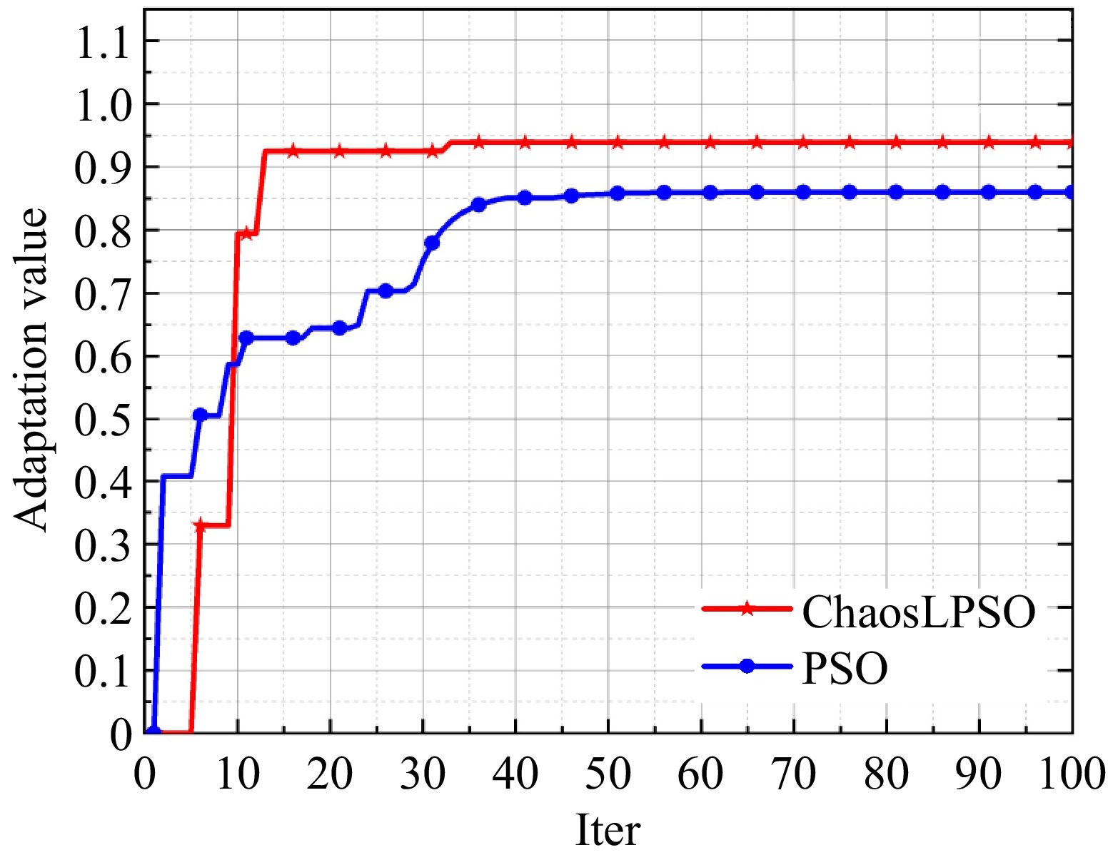
Figure 8. 

Comparison of the ChaosLPSO algorithm with the PSO algorithm.

From Fig. 8, it can be observed that the traditional PSO algorithm has a slower convergence rate, converging to the maximum fitness (85.9%) after 40 iterations. In contrast, the ChaosLPSO algorithm exhibits a faster convergence rate, converging to the maximum fitness (93.9%) after 32 iterations. The optimal system parameters at the maximum fitness are: f = 84.863 kHz, n = 0.2465. Since f/f₀ ≈ 1, the system operating frequency f is selected to be 85 KHz. The optimized parameters are as follows: L_f = 17.27 μH, C_f = 21.22 nF, and C₁ = 65.19 nF. Considering the stochastic nature of population distribution in the algorithm, both algorithms were computed three times, and the number of iterations to converge to the maximum fitness was recorded using a timer in MATLAB. The simulation results are recorded in Table 2.

Comparing the results of the two algorithms, it can be seen that the ChaosLPSO algorithm avoids the population getting trapped in local optima during the iteration process, allowing for rapid convergence.

Simulation verification

In Simulink, an LCC-S system model was established, and through simulation, ChaosLPSO, PSO, and initial parameters were validated.

From Fig. 9, it can be observed that the efficiency corresponding to the initial parameters and the improved algorithm is quite close and both are higher than the efficiency of the traditional algorithm. However, as seen in Table 3, the power corresponding to the improved algorithm is significantly higher than the power corresponding to the initial parameters, meeting the power constraint range. The parameters derived by the improved algorithm are better suited for the parameter settings of wireless power transfer systems. Set up five operational modes: the first one as the initial parameters, the second one as parameters optimized by PSO, the third one as parameters optimized by ChaosLPSO, the fourth one as the parameters of ChaosLPSO optimization with the load changed to 2Ω while keeping other parameters constant, and the fifth one as the parameters of ChaosLPSO optimization with the load changed to 20Ω while keeping other parameters constant. Perform simulation validation and comparison among the five operational modes.

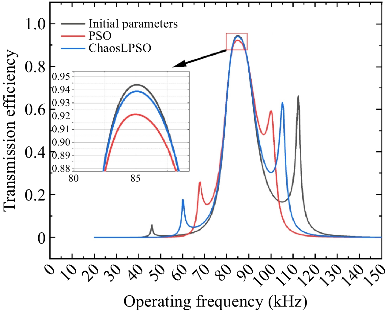
Figure 9. 

Effect of operating frequency on transmission efficiency.

Based on the simulation results shown in Fig. 10, the table below investigates the system transmission efficiency and output power in each operating mode before and after optimization configuration, as shown in Table 3. Although the transmission efficiency under the initial parameters is quite high, the output power does not meet the requirements. The parameters optimized through PSO fall into a local optimum, with a transmission efficiency of less than 90%. The parameters optimized by ChaosLPSO achieve maximum transmission efficiency while satisfying the output power requirements. Upon changing the load size, the output power and transmission efficiency follow the variations depicted in Fig. 5. When the load decreases from 10 to 2 Ω, the output power increases while the transmission efficiency decreases. Conversely, when the load increases from 10 to 20 Ω, the output power decreases, but the initial efficiency improves. By comparing the output power and transmission efficiency of operating modes 3, 4, and 5, it is evident that a load of 10 Ω is more suitable. Mode 1 presents the simulation results of the initial set parameters, while Mode 2 shows the simulation results after parameter optimization using the particle swarm optimization algorithm. Mode 3 reflects the simulation results after optimization with the improved particle swarm optimization algorithm. Modes 4 and 5 display the simulation results based on Mode 3 with changes made to the load.

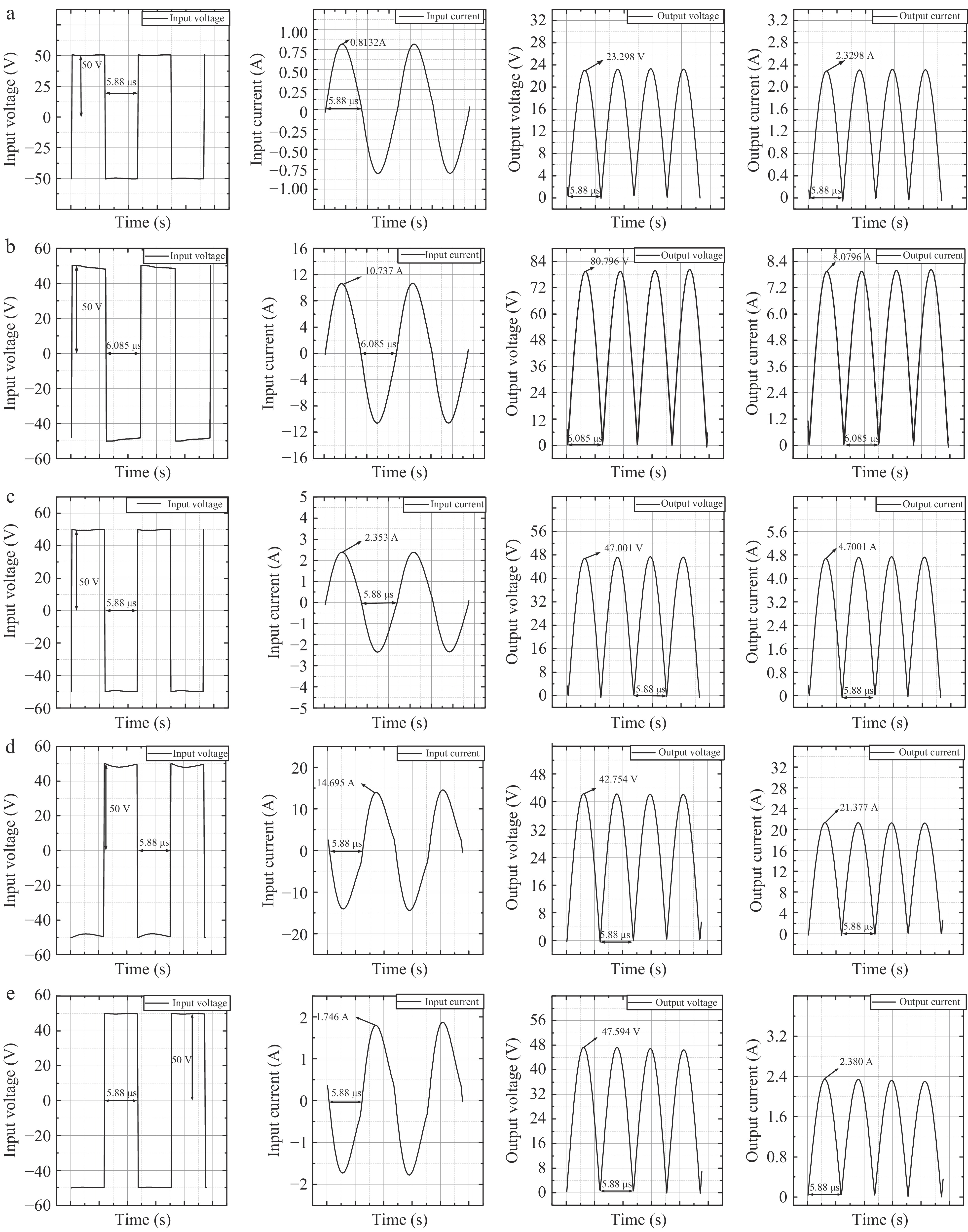
Figure 10. 

Simulation diagrams of the five operational modes. (a) Operating mode 1; (b) Operating mode 2; (c) Operating mode 3; (d) Operating mode 4; (e) Operating mode 5.

To verify whether the stress of the optimized devices complies with the constraints, a simulation was conducted in Simulink. The results of the experimental verification of the stress of the device are shown in Figs 11 and 12. Figure 11 represents the voltage stress graph, indicating that the self-inductance voltage (201.39 V) in the transmitting resonant coil in the device is at its maximum and below the maximum constraint voltage (300 V), satisfying the constraints.

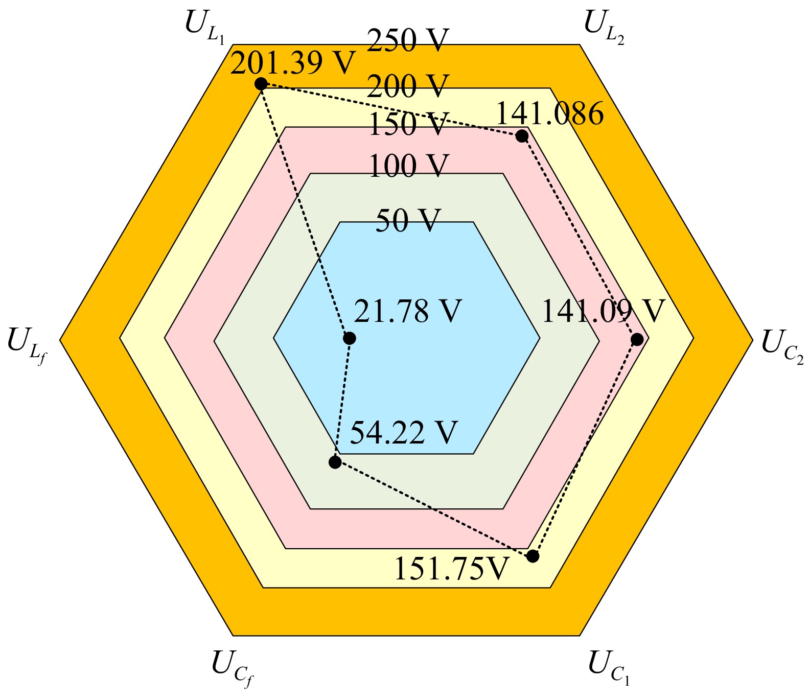
Figure 11. 

Simulation results of the voltage of components.

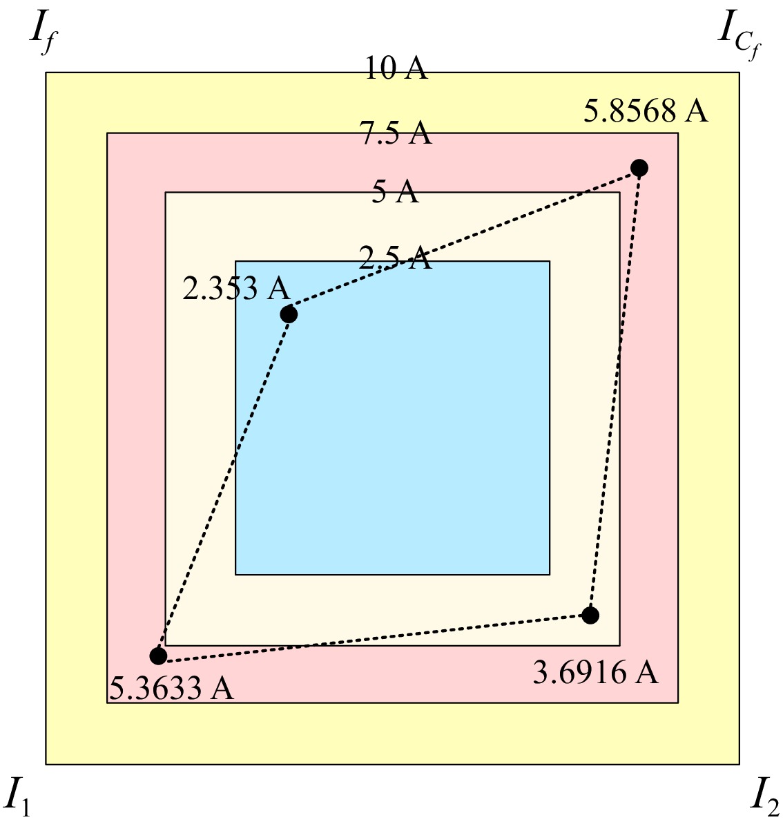
Figure 12. 

Simulation results of the current of components.

Experimental verification

To further validate whether the results optimized by the algorithm meet the requirements, experimental verification was conducted. The experimental platform is shown in Fig. 13. Some parameters are referenced from Table 1, and the working frequency, compensation inductance L_f, and compensation capacitance C_f are set according to the optimization results.

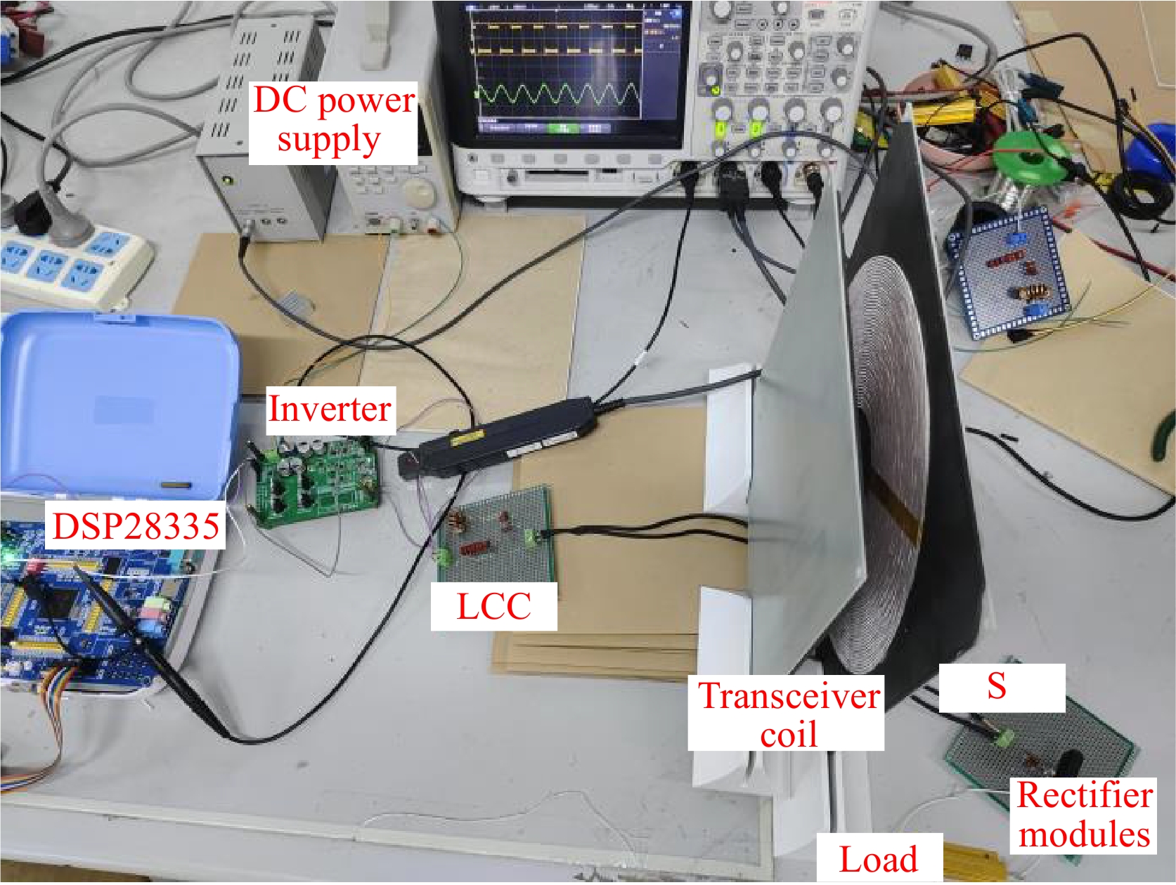
Figure 13. 

The wireless charging experimental platform.

Measurements of the inverter voltage and current waveforms for output voltage and current, are shown in Fig. 14.

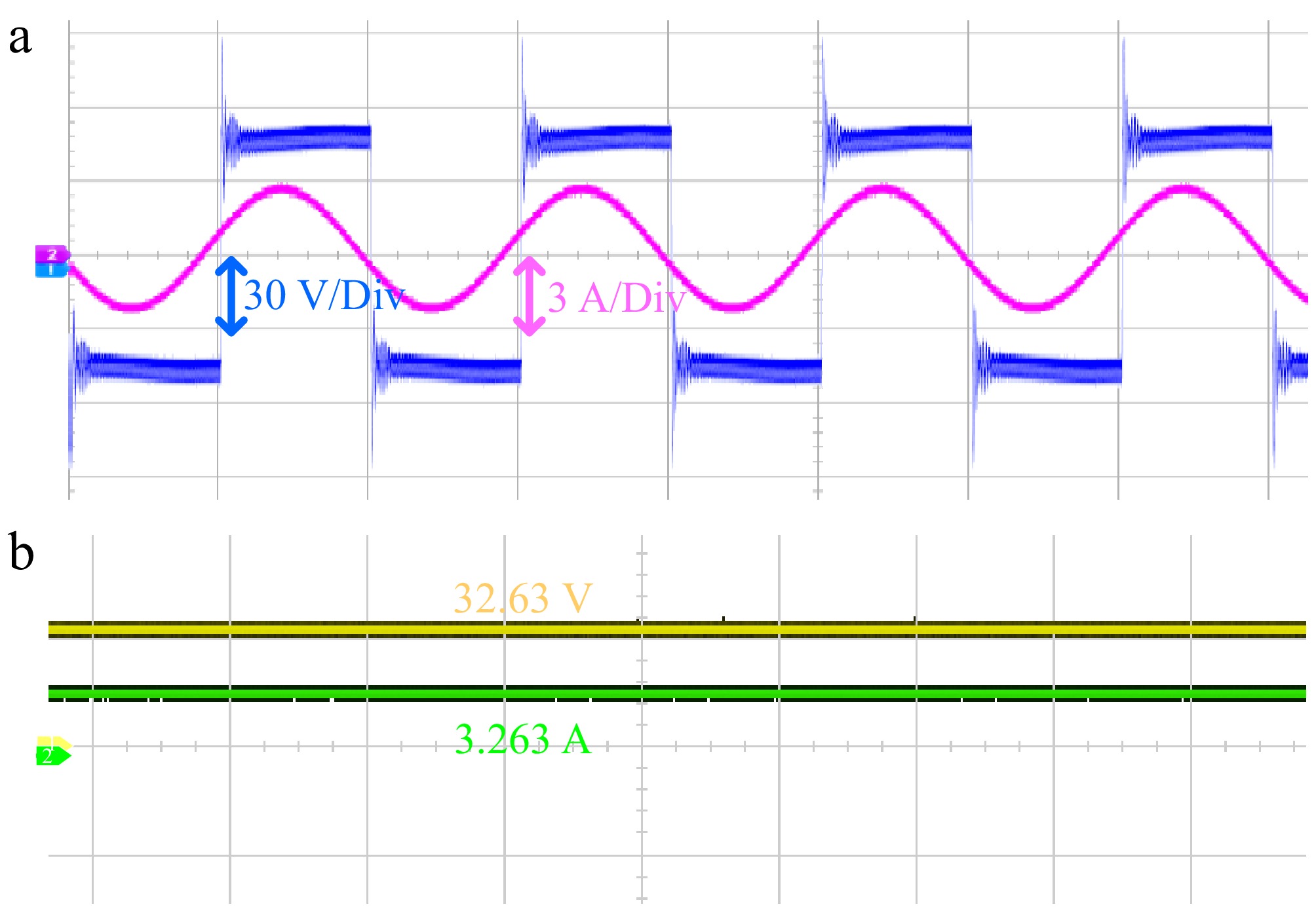
Figure 14. 

Experimentally measured voltage and current waveforms. (a) Input voltage and current, (b) Output voltage and current.

The output voltage and current are measured values after the filter capacitor, and based on the data in Fig. 14, the output power can be calculated as 108.36 W and the transmission efficiency as 92.11%. Although there is an error compared to the simulation, it is in line with the range of power and the efficiency is higher than 90%.

To verify that the stresses of the experimental equipment are in accordance with the constraints, voltage measurements, and current measurements are performed on individual components. The measurements of the stresses of the experimental setup are shown in Fig. 15.

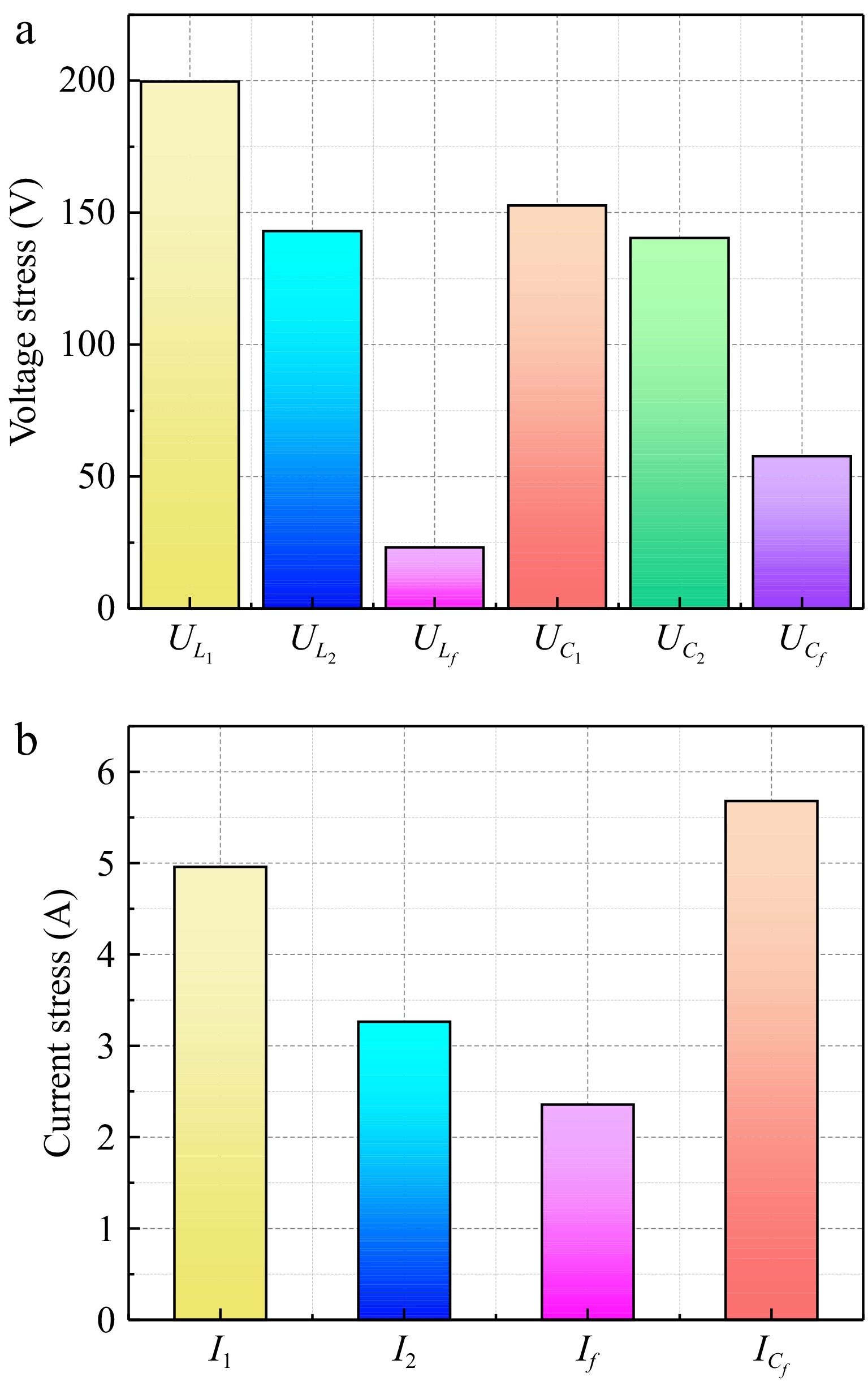
Figure 15. 

Voltage and current values of components. (a) Component voltage value, (b) component current value.

From Fig. 15 it is evident that the voltage values in the experiment are less than 1 kV and the current values are less than 10 A, which satisfies the constraints.

The five modes of the simulation were experimentally verified and the experimental results are shown in Table 4. Due to certain errors in the experimental process, the transmission efficiency and output power of the experimental results are low, but mode 3 meets the requirements of efficiency and power, and the experimental results are consistent with the simulation results.

This paper presents an improved PSO algorithm that incorporates chaotic mapping (Logistic) in population initialization and uses an enhanced Lévy flight mechanism to update particle positions. The effectiveness of the improved algorithm is validated based on Matlab simulation results. When comparing the traditional PSO algorithm with the improved PSO algorithm, the results indicate that the improved PSO algorithm optimizes higher transmission efficiency. Furthermore, the output power corresponding to the parameters optimized by the improved PSO algorithm is higher than the output power for parameters optimized by the traditional PSO algorithm and the initial parameters. An analysis of the transmission performance before and after system optimization was conducted. Through simulation and experimental verification, it is found that the optimization method improves the transmission performance of the system.