


-
Wireless power transmission (WPT) technology has been a hot research topic in the last decade due to its flexibility, low maintenance, and safety[1]. These systems have formed the basis for various industrial applications and interdisciplinary fields, such as wireless charging for electric vehicles[2,3], wireless motors[4−6], wireless lighting[7], wireless energy-on-demand[8], wireless power encryption[9], and wireless power trading[10]. It is widely used in the medical field, consumer electronics, household appliances, and electric vehicles[11,12].
There are multiple parameter variations in the application of WPT and this paper aims to study wireless charging in electric vehicles. When the deviation of the parking position of the electric vehicle and the difference in the height of the vehicle chassis will affect the change of the coupling coefficient and lead to the change of mutual inductance[13,14], as well as the equivalent impedance of the vehicle's energy storage battery will increase with the charging time during the charging process, which will lead to the decrease of the charging efficiency[15]. The parameter identification technique is beneficial to the development of appropriate control strategies to maintain the stability and efficiency of the system.
At present, some scholars have carried out related research around the problem of identifying the load and mutual inductance parameters of WPT systems. When the system does not use a modulation strategy, some researchers use a primary-side open-ended capacitor to ensure that the receiver-side reflected impedance at three frequencies can form the imaginary part of the input impedance, and then the voltage and current are collected to complete the identification of the system parameters[16]. Some researchers use the method of switching circuits to short-circuit the compensation network at the receiving end, and then obtain the phase information of the output voltage and current of the inverter by the method of sweeping to realise the identification of the parameters[17]. Some researchers propose a parameter identification method based on impedance matching, which parameterises different circuit models according to loads of different natures, obtains the parameter relationship between the transmitter and the load, and completes the parameter identification[18]. Each of these methods requires the addition of extra circuitry, which increases the cost and is only applicable to parameter identification for one topology.
In terms of different modulation strategies applied, some researchers proposes a WPT load parameter identification method by DC input current and phase shift angle. Due to the phase shift control used in the controller, the phase shift angle can be easily calculated, and the identification of the parameters can be accomplished simply by collecting the input current at the transmitter side[19]. A parameter identification method based on pulse density modulation (PDM) is proposed, in which a series of interharmonics are obtained by varying the sequence of the PDM, a system of equations is constructed using the simple harmonic waves, and finally, the load and mutual inductance are estimated using the least-squares approximation[20]. However, both PSC and PDM have a non-negligible problem, that is, PSC has high switching loss and is not easy to achieve zero voltage switching (ZVS); PDM can easily achieve ZVS, but the output fluctuation is large. Moreover, the identification method is very complicated due to the application of the modulation method.
Intelligent algorithm technology has been developing rapidly in recent years, and researchers have begun to apply AI algorithms to WPT systems to solve the problem of mutual inductance and load identification[21]. In this paper, a parameter identification method based on the Improved Northern Goshawk Optimization (INGO) Algorithm is proposed, which converts parameter identification into an optimal problem, and accurate identification of mutual inductance and load can be accomplished by collecting the output current of the inverter, and the proposed identification method is applied to the WPT system that incorporates the pulse frequency control strategy, and achieves the maximum efficiency tracking of the WPT system through impedance matching.
Compared to existing methods, the main contributions of this paper are as follows:
An Improved Northern Goshawk Optimization (INGO) Algorithm is proposed, which introduces an optimal value guidance strategy, a subtraction optimizer, and Cauchy mutation to enhance the global convergence speed and the ability to escape local optima. This improvement makes the parameter identification process more efficient and accurate, especially under conditions of load variation, and coil misalignment.
The proposed method integrates the parameter identification process with the Pulse Frequency Modulation (PFM) strategy, which effectively reduces switching frequency and switching losses while suppressing output fluctuations. Compared to traditional Phase Shift Control (PSC) and Pulse Density Modulation (PDM), PFM simplifies the control strategy and reduces the complexity of parameter identification.
Beyond parameter identification, this paper achieves maximum efficiency tracking through a Sepic impedance matching circuit, ensuring that the system maintains maximum transmission efficiency even under load variations and coil misalignment.
The proposed method significantly reduces hardware complexity and system cost by eliminating the need for additional circuits or complex control strategies, as required in traditional methods[16, 17].
We begin by analyzing the system topology and the principle of operation, followed by an introduction to the basic principles of the PFM modulation strategy. Additionally, the calculation method for the output current of the inverter circuit after applying the PFM modulation strategy is presented. The relationship between mutual inductance and the basic parameters of the circuit is derived, and the load and mutual inductance are identified using the measured current on the transmitter side. Finally, the conditions required for the Sepic circuit to achieve the maximum efficiency of the system are derived.Next, an INGO algorithm is proposed, which enhances the algorithm's ability to escape local optima and accelerates the speed of global convergence. The entire identification process is described in detail. The feasibility of the proposed INGO algorithm for parameter identification is then verified through simulation and experimental results.In conclusion, the effectiveness of the method and its practical applications are summarized.
-
Due to its advantages such as simple structure, strong stability, and ease of control, the SS-type topology is widely used in electric vehicles and medical electronics[22]. Therefore, this paper analyzes and discusses the SS-type topology. Figure 1 shows the equivalent circuit diagram of the SS-type topology.
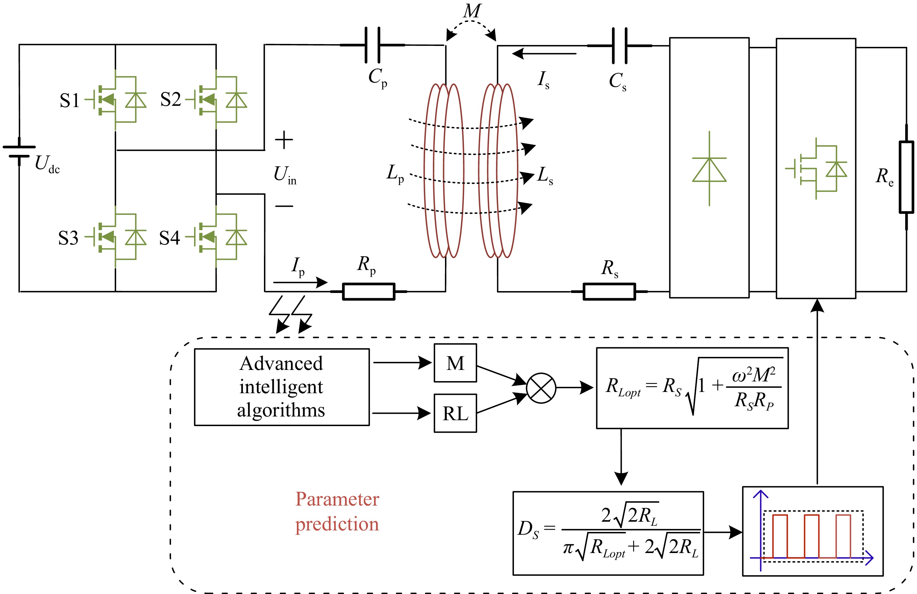
Figure 1.
SS type topology structure input by inverter.
Udc is the DC voltage input to the system. S1~S4 is a full-bridge inverter circuit composed of four mosfets, which can generate an approximate square-wave input AC voltage Uin by alternating the conduction of two groups of switching tubes, and Ip is the input AC current after inversion. Lp and Ls are the self-inductances of the transmission coils on the transmitter and receiver, respectively. Cp and Cs are the resonant compensation capacitors on both sides. Rp and Rs are the equivalent series resistances on both sides. Re = 8RL/π2 represents the equivalent resistance of the load and rectifier circuit on the receiver side, while the load RL varies with the charging time. The mutual inductance M between the transmission coils is M = k(LpLs)1/2. Where k is the coupling coefficient between the coils, when the coils are offset k changes resulting in a change in the M.
Since the reactive power can be minimised when the system operates at the resonant frequency, the operating frequency ω of the system can be set to approximate the resonant frequencies ωp and ωs. The operating frequency ω is given by Eqn (1).
$ \omega \approx {\omega _P} \approx {\omega _S} \approx \frac{1}{{\sqrt {{L_{\text{p}}}{C_p}} }} \approx \frac{1}{{\sqrt {{L_{\text{s}}}{C_{\text{s}}}} }} $ (1) At this point, the WPT system circuit equation is:
$ \left\{ \begin{gathered} {U_{in}} = \left( {{R_P} + j{X_{P\_n}}} \right){I_p} + j\omega M{I_s} \\ 0 = j\omega M{I_p} + ({R_s} + {R_e} + j{X_{s\_n}}){I_s} \\ \end{gathered} \right. $ (2) where, Xp_n and Xs_n are the reactances under the excitation of the nth harmonic voltage at the output of the inverter on the transmitter and receiver sides, respectively.
$ \left\{ \begin{gathered} {X_{p\_n}} = n\omega {L_p} - \dfrac{1}{{n\omega {C_p}}} \\ {X_{s\_n}} = n\omega {L_s} - \dfrac{1}{{n\omega {C_s}}} \\ \end{gathered} \right. $ (3) The input impedance can be expressed as
$ {Z}_{i{n}_{n}}={a}_{n}+{jb}_{n} $ $ \left\{ \begin{gathered} {a_n} = {R_p} + \dfrac{{{n^2}{\omega ^2}{M^2}({R_s} + {R_e})}}{{{{({R_s} + {R_e})}^2} + X_{s\_n}^2}} \\ {b_n} = X_{p\_n}^2 - \dfrac{{{n^2}{\omega ^2}{M^2}{X_{s\_n}}}}{{{{({R_s} + {R_e})}^2} + X_{s\_n}^2}} \\ \end{gathered} \right. $ (4) The transmission efficiency of the system is obtained from Eqn (2) as:
$ \eta = \dfrac{{{\omega ^2}{M^2}{R_e}}}{{\left( {{R_s} + {R_e}} \right)\left( {{R_p}\left( {{R_s} + {R_e}} \right) + {\omega ^2}{M^2}} \right)}} $ (5) To achieve maximum efficiency transmission we need to optimise the load resistance. So the efficiency η can be calculated as a differential with respect to Re. When the system satisfies the maximum efficiency transmission, the optimum load resistance is:
$ {R_{eopt}} = {R_S}\sqrt {1 + \dfrac{{{\omega ^2}{M^2}}}{{{R_S}{R_P}}}} $ (6) Pulse frequency modulation
-
To enhance the efficiency and stability of WPT systems and meet the demands under various operating conditions, modulation strategies are often implemented in the full-bridge inverter circuit on the transmitter side. Pulse Frequency Modulation (PFM) has become a focus of research due to its alternating modulation at two different frequencies and its ability to easily achieve soft switching. Compared to traditional Phase Shift Control (PSC), PFM effectively reduces switching frequency and switching losses. Furthermore, compared to Pulse Density Modulation (PDM), PFM not only reduces switching frequency but also effectively suppresses output fluctuations. Figure 2 illustrates the theoretical modulation waveform of PFM.
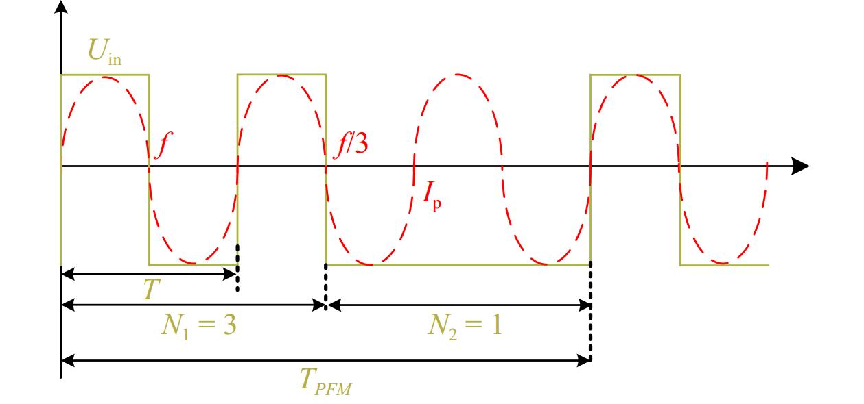
Figure 2.
PFM theoretical modulation waveform.
In PFM, the system alternates modulation between two different frequencies, f and f/3. Here, N1 represents the number of square waves at the switching frequency f, and N2 represents the number of square waves at the switching frequency f/3. The PFM control of the inverter output is essentially a piecewise function, which can be expressed in its Fourier series form as:
$ {U_{in}}(t) = \left\{ {\begin{array}{*{20}{c}} {\dfrac{{4E}}{\text π}\sum\limits_{{n_F}}^\infty {\dfrac{{\sin \left[ {\left( {2{n_F} - 1} \right){\omega _{2n - 1}}t} \right]}}{{2{n_F} - 1}}} }&{{\omega _{2n - 1}} = \dfrac{\omega }{{2n - 1}}} \\ {\dfrac{{4E}}{\text π}\sum\limits_{{n_F}}^\infty {\dfrac{{\sin \left[ {\left( {2{n_F} - 1} \right){\omega _{2n + 1}}t} \right]}}{{2{n_F} - 1}}} }&{{\omega _{2n - 1}} = \dfrac{\omega }{{2n + 1}}} \end{array}} \right. $ (7) where, ω2n±1 are the modulating angular frequencies of the two segmented output voltages, and by selecting the output vectors generated by two neighbouring (2n ± 1) harmonics, the target vector with the minimum output fluctuation can be synthesized. The WPT system is driven by the odd harmonic segments since the odd harmonic frequencies of the two segmented function outputs are equal to the system operating frequency. The characteristics of the system are determined by its fundamental components, so the average Fourier series expansion of the fundamental components of the output voltage of the PFM inverter is as follows[23]:
$ \begin{aligned} U{}_{in\_1}(t) =\;& \dfrac{{\alpha {n_1}}}{{\alpha {n_1} + (1 - \alpha ){n_2}}}\dfrac{{4U}}{{{n_1}{\text π} }}\sin ({n_1}{\omega _{2n - 1}}t) \\ & + \dfrac{{(1 - \alpha ){n_1}}}{{\alpha {n_1} + (1 - \alpha ){n_2}}}\dfrac{{4U}}{{{n_2}{\text π} }}\sin ({n_2}{\omega _{2n + 1}}t) \\ = \;&\dfrac{1}{{\alpha {n_1} + (1 - \alpha ){n_2}}}\dfrac{{4U}}{\text π}\sin (\omega t) \\ \end{aligned} $ (8) where, n1 = 2n − 1, n2 = 2n + 1. α = N1/(N1 + N2) is the control variable duty cycle factor of PFM. The transmitter side current can be expressed as:
$ {i_p}(t) = \dfrac{{{U_{in\_1}}(t)}}{{{Z_{in\_n}}}} = {I_n}\sin (\omega t) $ (9) where, In is the peak value of the nth harmonic of the inverter output current:
$ \begin{aligned} {I_n} =\;& \dfrac{1}{{\alpha {n_1} + (1 - \alpha ){n_2}}}\dfrac{{4U}}{{{\text π} \left| {{Z_{in\_n}}} \right|}} \\ = \;&\dfrac{1}{{\alpha {n_1} + (1 - \alpha ){n_2}}}\dfrac{{4U}}{{{\text π} \sqrt {a_n^2 + b_n^2} }} \\ \end{aligned} $ (10) By bringing Eqn (3) into Eqn (9), one can solve for:
$ M = \dfrac{1}{\omega }\sqrt {{X_{p\_1}}{X_{s\_1}} - {R_p}{R_e} + \sqrt {{{\left( {\dfrac{{4U}}{{{\text π} {I_n}}}} \right)}^2}(R_e^2 + X_{s\_1}^2) - {{({X_{p\_1}}{R_e} + {X_{s\_1}}{R_p})}^2}} } $ (11) The initial steady state period after the system enters the steady state for the first time is denoted as TPFM_0, then TPFM_0 = nTPFM. By collecting the current at the moment of TPFM_0 on the transmitter side and constructing the fitness function with the current obtained from the computation of Eqn (10), the identification of the variations of the parameters M and RL can be carried out in the algorithm.
Maximum efficiency tracking
-
Impedance matching technology can be mainly divided into two implementation methods: passive and active. The passive impedance matching method uses combinations of capacitors and inductors in series and parallel to transform the load impedance, ensuring that the imaginary part of the equivalent impedance is zero while the real part matches the system's optimal load. However, this method can result in complex circuit structures when attempting to match arbitrary loads. Moreover, in practical applications, the load resistance typically varies dynamically, and the parameters of passive impedance matching networks are difficult to adjust in real-time, making it challenging to adapt to these dynamic changes and limiting the system's efficiency optimization capabilities. In contrast to passive impedance matching, the active impedance matching method can dynamically adjust the secondary-side equivalent impedance by adjusting the duty cycle of a DC-DC converter, without the need to change system component parameters. This effectively overcomes the limitations of passive matching and optimizes system efficiency.
As shown in Table 1, the Sepic converter offers significant advantages in impedance matching applications within wireless charging systems due to its wide input-output voltage range, stable voltage polarity, efficient power transfer, and good current matching capabilities. Therefore, this paper selects the Sepic converter to implement the system's maximum efficiency tracking, and its topology is shown in Fig. 3.
Table 1. Comparison of five basic DC-DC converters
Characteristic Sepic Boost Buck-Boost Cuk Zeta The range of Req 0 ~ $ + \infty $ 0 ~ RL 0 ~ $ + \infty $ 0 ~ $ + \infty $ 0 ~ $ + \infty $ The polarity of US/Uo Same Same Reverse Reverse Reverse Conversion efficiency Higher higher medium medium medium Input current continuity Continuous Discontinuous Discontinuous Continuous Continuous Cost medium Lower medium higher higher 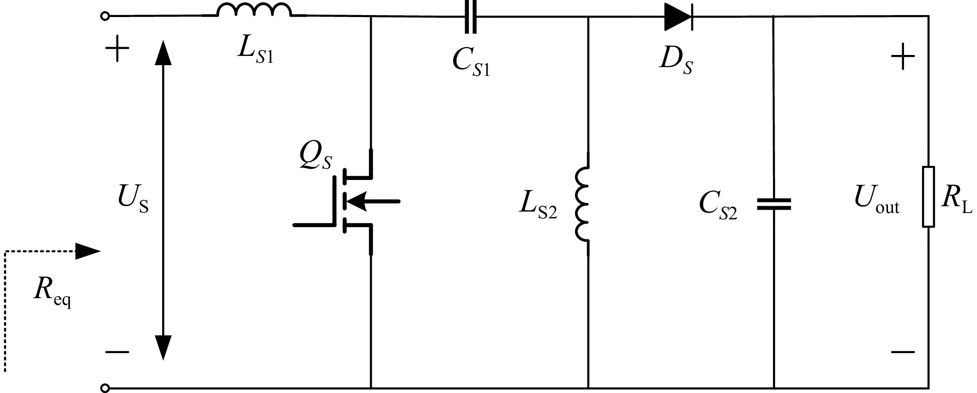
Figure 3.
Receiver added to the Sepic circuit.
The input and output voltages of the Sepic circuit are related to the equivalent resistance as follows:
$ \dfrac{{{U_S}^2}}{{{R_{eq}}}} = \dfrac{{{U_{out}}^2}}{{{R_L}}} $ (12) Assuming that the duty cycle of switching tube QS in the Sepic circuit is DS, then:
$ {U_{out}} = \dfrac{{{t_{on}}}}{{{t_{off}}}}{U_E} = \dfrac{{{t_{on}}}}{{T - {t_{on}}}}{U_E} = \dfrac{{{D_S}}}{{1 - {D_S}}}{U_E} $ (13) The relationship between the equivalent resistance Req and the duty cycle DS in the Sepic circuit is given by:
$ {R_{eq}} = {(\frac{{1 - {D_S}}}{{{D_S}}})^2}{R_L} $ (14) The system receiver impedance Re with duty cycle DS can be derived as:
$ {R_e} = \dfrac{8}{{{{\text π} ^2}}} \times {\left(\dfrac{{1 - {D_S}}}{{{D_S}}}\right)^2}{R_L} $ (15) For a determined static WPT system has a unique best load value, so that Re = Reopt, the system load resistance RL and duty cycle DS when the system is at the point of maximum transmission efficiency is obtained as:
$ {D_S} = \dfrac{{2\sqrt {2{R_L}} }}{{\pi \sqrt {{R_{eopt}}} + 2\sqrt {2{R_L}} }} $ (16) -
The Northern Goshawk Optimization Algorithm is a population-based optimisation algorithm that is conceived through the hunting strategy of the Northern Goshawk[24]. The hunting of the Northern Goshawk consists of two phases: prey recognition and attack and chase and escape, in the first phase, after recognising the prey it moves towards it at high speed, and in the second phase it hunts the prey with a short tail chase process. The Algorithm simulates the hunting process of the Northern Goshawk.
Introducing an optimal value guidance strategy
-
In the first stage of the prey escape process of NGO, when
$ {F}_{{P}_{i}} < {F}_{i} $ $ {x_{i,j}} + q({x_{best}} - I{x_{i,j}}),{F_{{G_i}}} \lt {F_i} $ (17) Introduction of subtraction algorithm of optimizer
-
In the first stage of the NGO, during the prey escape process, when
$ {F}_{{G}_{i}} > {F}_{i} $ $ {x_{new1,i,j}} = \left\{ {\begin{array}{*{20}{c}} {{x_{i,j}} + q({x_{best}} - I{x_{i,j}})}&{{F_{{G_i}}} \lt {F_i}} \\ {{x_{i,j}} = {x_{i,j}} + \vec q\frac{1}{N}\sum\limits_{K = 1}^N {({x_i} - {}_v{x_k})} }&{{F_{{G_i}}} \geqslant {F_i}} \end{array}} \right. $ (18) From Eqn (18), it can be seen that the subtractive optimiser will synthesise the global position which is constantly updated, which, to some extent, enhances the likelihood of the algorithm jumping out of the local optimum and accelerates the global convergence.
Adding probability factors for Cauchy variation
-
Adding a certain probability factor for Cauchy mutation in the 2nd stage of the NGO's Pursuit and Escape. The Cauchy variation formula is as follows:
$ {x_{newbest}} = {x_{best}} + {x_{best}}Cauchy\;(0,1) $ (19) Dynamic updating of position based on upper and lower bounds
-
In the 2nd stage of the NGO pursuit and escape, certain probability factors are added for Cauchy variation, and upper and lower limits are introduced for gradual reduction. This allows the NGO to dynamically shrink the target range as the number of iterations increases, accelerating the convergence ability of the Algorithm. The second stage of the improved formula is as follows:
$ {x_{new1,i,j}} = \left\{ {\begin{array}{*{20}{c}} {{x_{new2,i,j}} = {x_{best}} + {x_{best}}Cauchy(0,1)}&{rand \lt \sigma } \\ {{x_{new2,i,j}} = {x_{i,j}} + \dfrac{{r(2s - 1)(ub - lb)}}{t}}&{rand \gt \sigma } \end{array}} \right. $ (20) where, Cauchy(0,1) is the Cauchy variation and
$ \sigma $ $ rand < \sigma $ $ rand > \sigma $ Figure 4 shows the experimental plot of the proposed Algorithms in this paper in comparison with other Optimizations. Comparison with Subtractive Algorithm of Optimization (SAO) Sparrow Search Algorithm (SSA), Dung Beetle Optimization (DBO) Golden Jackal Optimization (GJO), and the original NGO shows the superiority of the INGO proposed in this paper in terms of speed of convergence as well as in terms of comparison of error.
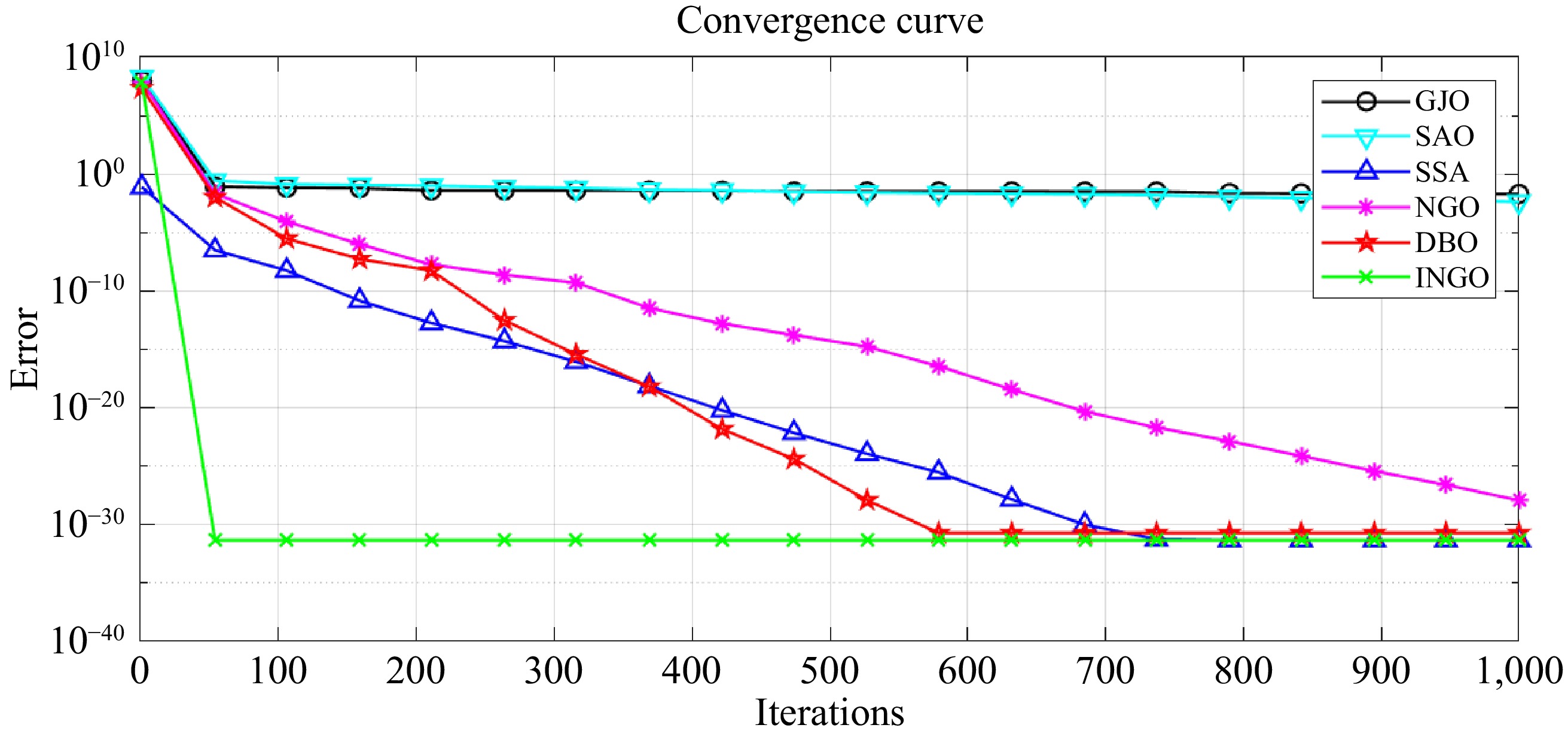
Figure 4.
Comparison of the performance of the optimization proposed in this paper with the remaining several optimizations.
Since particle swarm optimization (PSO) and genetic algorithms (GA) have been studied for a long time, this paper compares the proposed improved Northern Goshawk Algorithm (INGO) with more recent optimization algorithms, such as the Sparrow Search Algorithm (SSA) and the Scarab Beetle Algorithm (SAO), which are currently popular in the optimization field. Compared to other artificial intelligence algorithms, the INGO algorithm achieves a better balance between computational efficiency and recognition accuracy. INGO introduces several enhancement features, including optimal value guidance strategy, subtraction optimizer, and Cauchy mutation, all of which improve global exploration and local optimization. Although these features slightly increase the computational cost per iteration, INGO compensates for this by requiring fewer iterations. This makes INGO faster and more accurate, particularly in parameter identification problems in WPT systems. Table 2 shows a comparison between INGO and other algorithms with the same population size and iteration count. INGO typically converges in 100 iterations with an average recognition error of 1.2%, while DBO and SSA require 600 and 750 iterations with average errors of 1.5%. Although GJO and SAO converge quickly, their recognition accuracy is poor, with an average error of 3.8%.
Table 2. Comparison with other algorithms in parameter identification.
Algorithm Avg. error (%) Iterations Computation time (t/s) INGO 1.5% 87 50 SAO 3.8% 50 30 SSA 1.5% 49 110 DBO 1.5% 581 80 GJO 3.8% 726 30 Figure 5 shows a flowchart of the implementation of the proposed improved northern goshawk parameter identification method, which is described as follows:
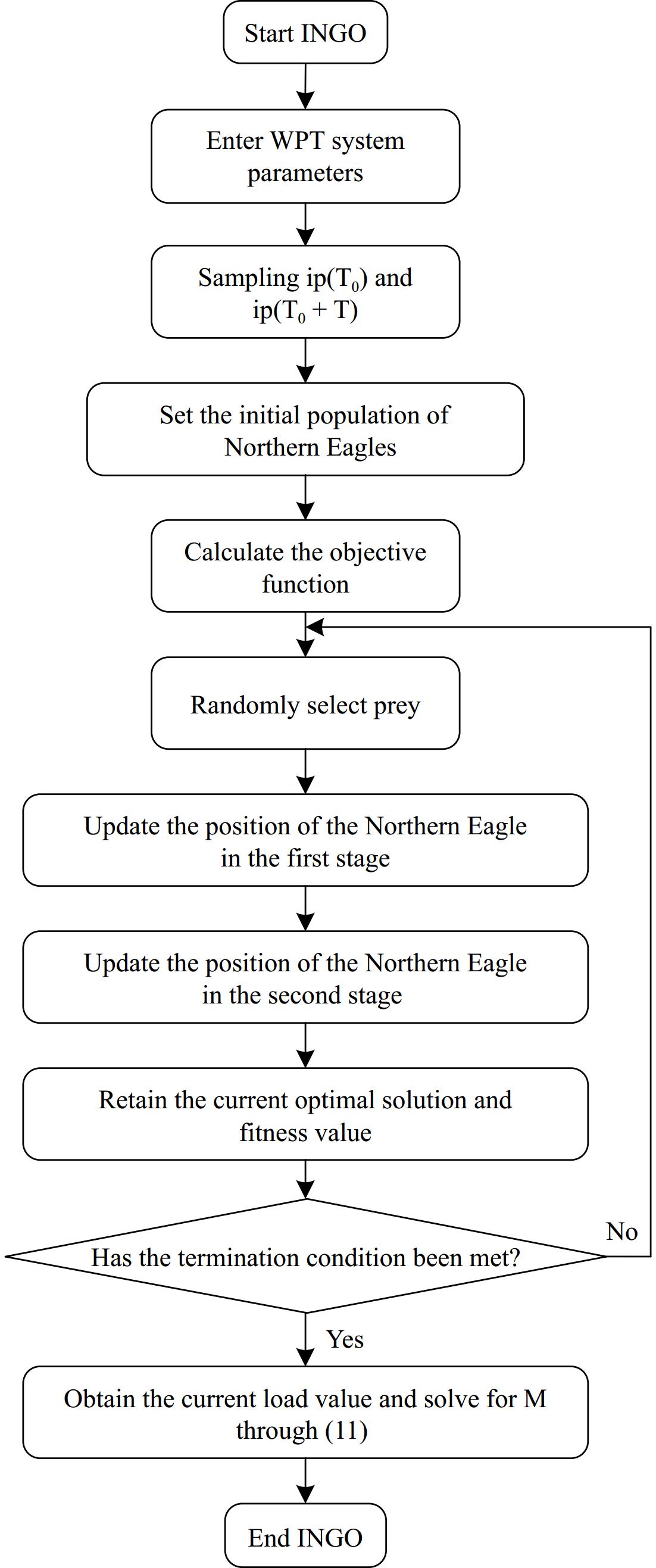
Figure 5.
INGO recognition flowchart.
(1) Input the system fixed parameter values (Udc, LP, LS, CP, CS, RP, RS), and parameterise the actual system model to get the transmitter side current i(TPFM_0) and measure the system i(TPFM_0)real during steady state operation.
(2) The initial population is generated according to the basic theory of the NGO. In this paper, the initial population size is set to 50, the load identification range is [0, 100 Ω], and the mutual sensing identification range is [0, 50 μH].
(3) The adaptation function is calculated by the error between the theoretical and actual values of the transmitter side currents and the result is used to reflect the similarity between the identified parameters and the actual parameters. The fitness function f(RL,M) is as follows:
$\begin{split}& f({R_{L,}}M) = \\&\sqrt {{{[i({T_{PFM\_0}}) - i{{({T_{PFM\_0}})}_{real}}]}^2} + {{[i({T_{PFM\_0}} + {T_{PFM}}) - i{{({T_{PFM\_0}} + {T_{PFM}})}_{real}}]}^2}}\end{split} $ (21) (4) Starting the execution of IGNO, updating the position of the northern Goshawk in the first and second phases. To determine whether the maximum number of iterations has been reached, or a predefined error is satisfied.
(5) The load optimal solution is obtained and solved to the M through Eqn (11), completing the whole identification process.
Experiment analysis and discussion
-
To verify the effective recognition results and feasibility of the proposed recognition method, we built the SS-WPT experimental platform as shown in Fig. 6, and the system parameters are shown in Table 3.
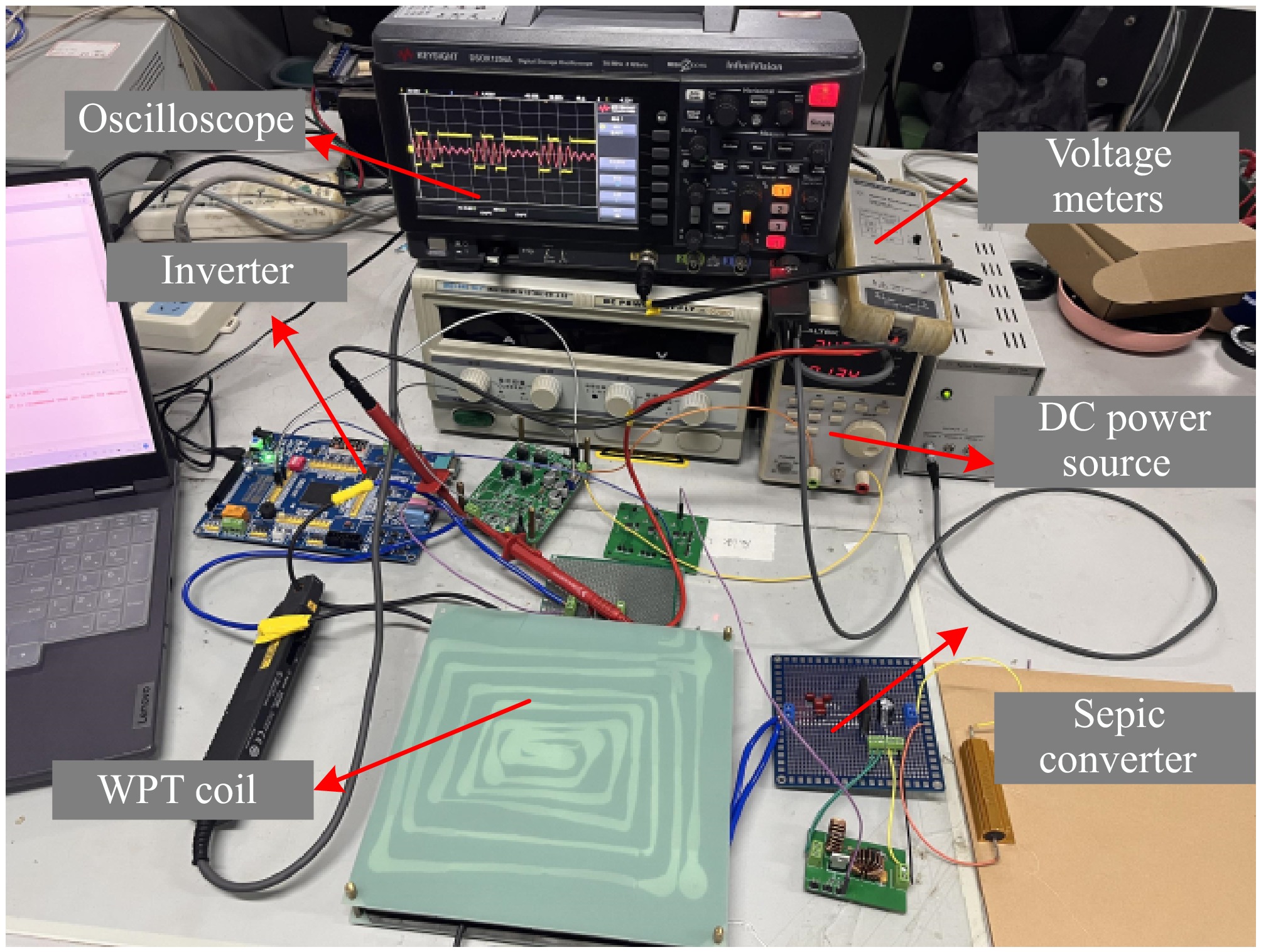
Figure 6.
Experimental model of the proposed WPT system.
Table 3. Design parameters and specifications.
Items Value DC input voltage (Udc) 24 V Transmitter compensated capacitance (CP) 16.5 nF Transmitter coil inductance (LP) 152.87μH Receiver compensated capacitance (CS) 16.49 nF Receiver inductances (LS) 153.6 μH Sepic inductances (LS1) 34.6 μH Sepic inductances (LS2) 33.4 μH Sepic compensated capacitance (CS1) 47 μF Sepic output capacitance (CS2) 2,200 μF Fundamental switching frequency (f) 100 kHz The detailed geometric shapes and dimensions of the transmitter-side and receiver-side coils are shown in Fig. 7a. Compared to fully wound planar spiral coils, the hollow planar spiral coils have a higher quality factor. The coil is made of 300 strands of Leeds wire with a total cross-sectional area of 2.35 mm2, 19 turns of dense winding, the outer diameter of the coil is 200 mm, the inner diameter of the coil is 140 mm, and the transmission distance is 70 mm. Ferrite strips, as well as an aluminium plate, are affixed on the coil to facilitate the increase of the coupling coefficient and the realization of the magnetic field shielding function, and the distribution of the magnetic field is shown in Fig. 7b.
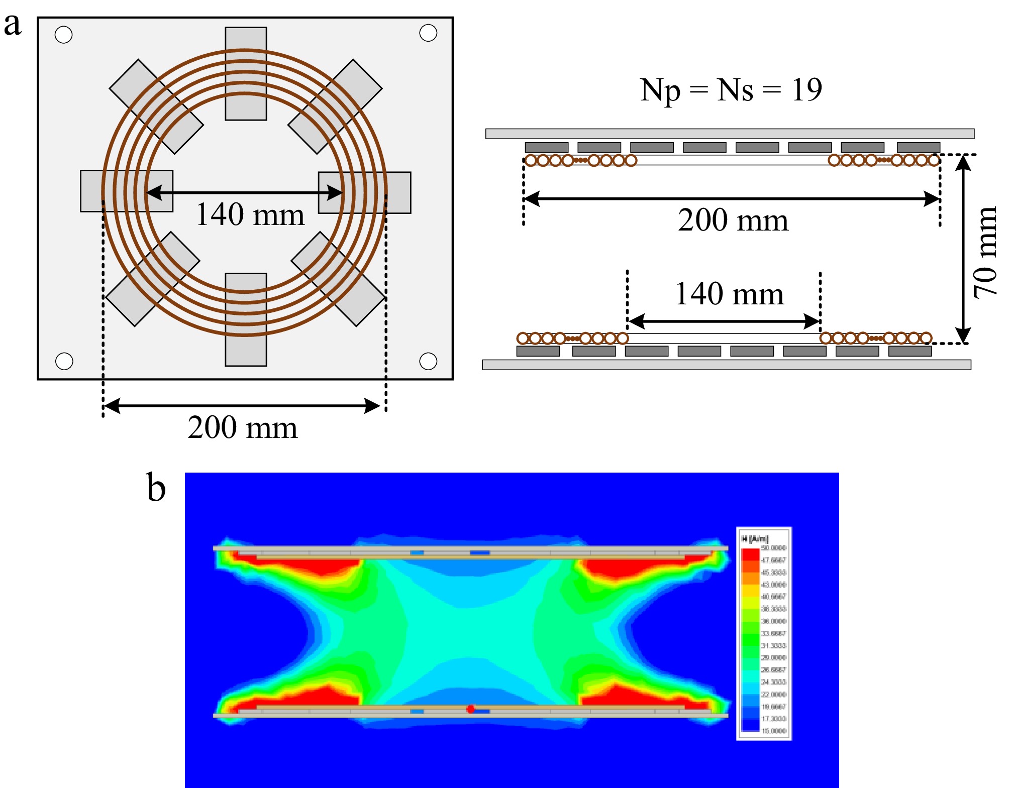
Figure 7.
(a) Transmitter and receiver side coil geometry. (b) Coil magnetic field distribution.
The actual measured values of the system load RL and mutual inductance M are 30 Ω and 34.97 μH, respectively, and the primary current is collected as the input condition of the Optimization, at this time, the circuit waveform is shown in Fig. 8.
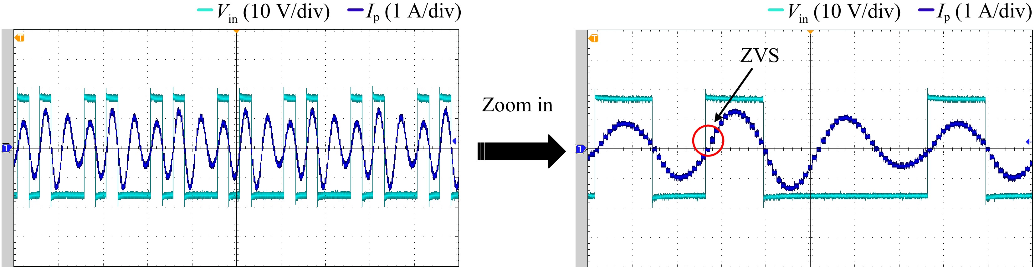
Figure 8.
Measured waveform of the PFM transmitter.
In view of the mutual inductance parameter changes due to coil offset during system operation, this paper analyses six sets of data without loss of generality, with the horizontal offset parameters to be identified as shown in Table 4 and the vertical offset parameters to be identified as shown in Table 5.
Table 4. Identification parameter value of mutual inductance parameter change.
0ffset (cm) R (Ω) M-x (μH) 1 30 34.14 2 30 33.01 3 30 30.95 4 30 28.41 5 30 25.47 6 30 22.35 Table 5. Identification parameter value of mutual inductance parameter change.
0ffset (cm) R (Ω) M-z (μH) −2 30 53.72 −1 30 43.49 1 30 28.95 2 30 23.93 3 30 19.17 4 30 16.47 Figure 9a shows the comparison between the actual and predicted values of mutual inductance when the receiving coil is horizontally shifted. Figure 9b shows the predicted parameter errors of the proposed method in this paper when the receiving coil is horizontally shifted, and the predicted error value is a maximum 3.039%, and a minimum 0.1% when the mutual inductance M is varied from 34.97 to 22.356 μH. Fixing the horizontal offset to zero and adjusting the position of the receiving and transmitting coils longitudinally along the z-axis, Fig. 10a shows the curve of the variation between the actual and predicted values of the mutual inductance M when the distance between the receiving and transmitting coils varies from 50 to 110 mm. The error between its predicted and actual values is given in Fig. 10b. It can be seen that the maximum error in the mutual inductance M prediction in terms of coil distance variation is 3.3% and the minimum error is 0.7%.
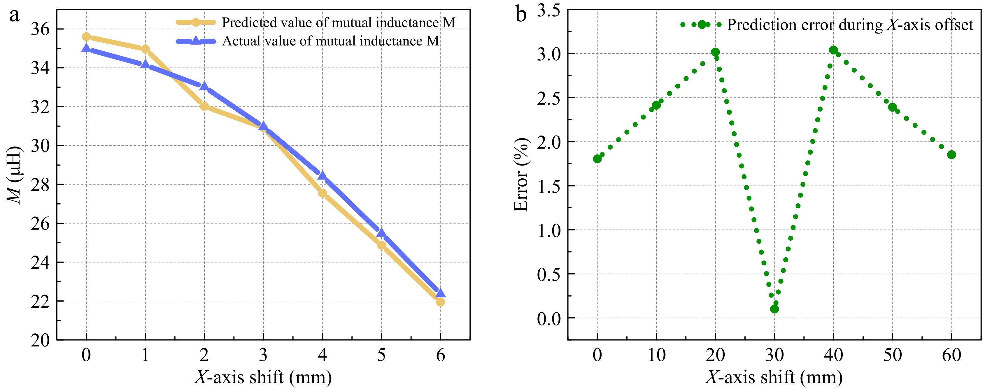
Figure 9.
Comparison between the actual value of mutual sensing and the recognition result at lateral offset. (a) Comparison of identified and actual values. (b) Error.
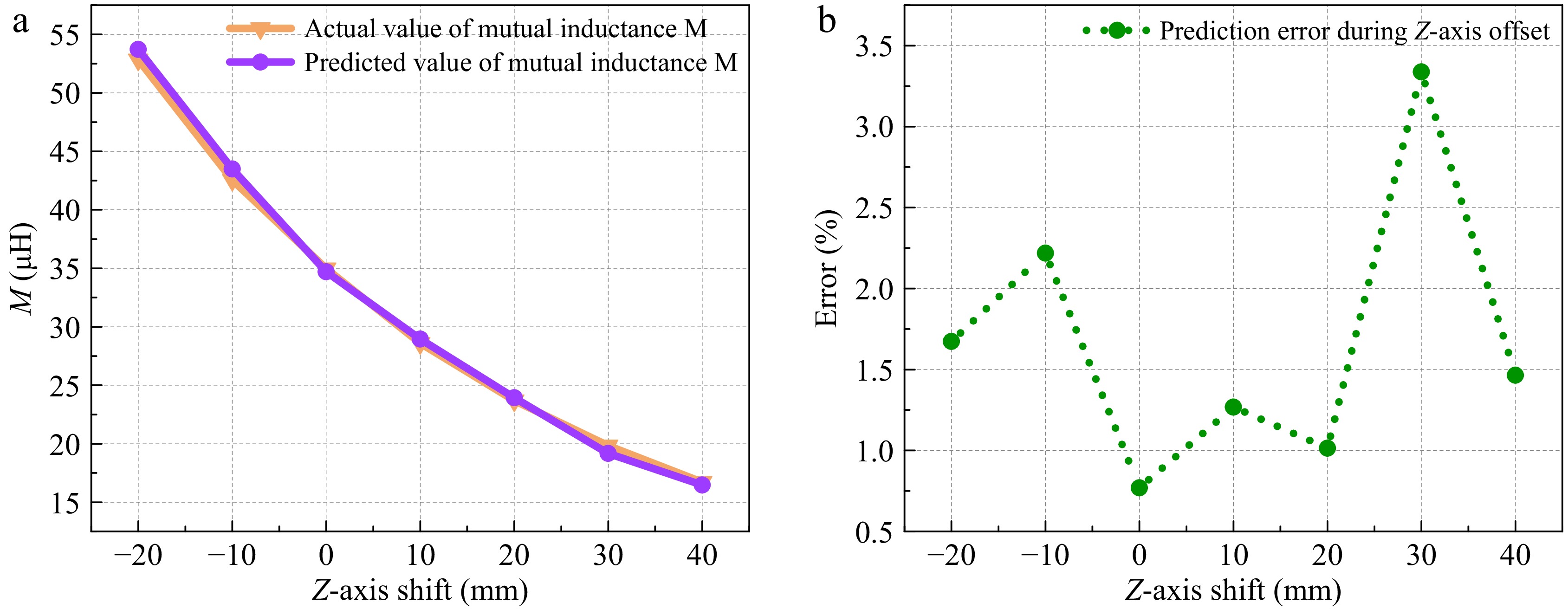
Figure 10.
Comparison between the actual value of mutual sensing and the recognition result at longitudinal offset. (a) Comparison of identified and actual values. (b) Error.
Because the load parameters may change during the operation of the system, this paper analyses the five groups of data without loss of generality, and the actual values of the four groups of parameters to be identified are shown in Table 6.
Table 6. Identification of parameter values for load parameter variations.
Case R (Ω) M (μH) 1 10 34.97 2 30 34.97 3 50 34.97 4 70 34.97 5 90 34.97 Figure 11a shows the comparison between the system identification value and the predicted value when the load changes, when the
$ {R}_{L} $ 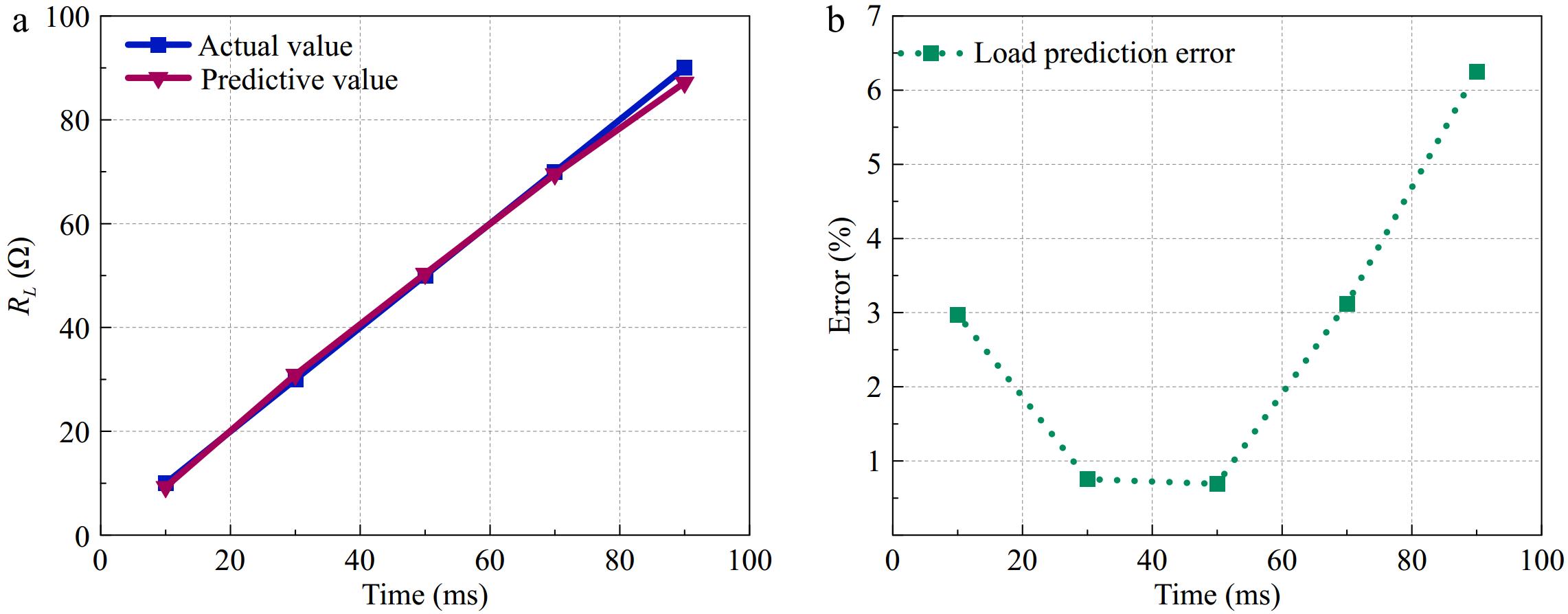
Figure 11.
Comparison of recognised values with actual values when the load changes (a) Comparison of identified and actual values. (b) Error.
The recognition effectiveness of the NGO algorithm is compared with that of the INGO algorithm under the same recognition parameters. The values of load RL and mutual inductance M are set to be 30 Ω, 34.97 μH, and 28.954 μH, respectively. The two algorithms are used to perform recognition six times and their errors are averaged. Figure 12a depicts the comparison of the average error between the INGO algorithm and the recognition effect of the NGO algorithm, and it can be seen that after the introduction of the optimal bootstrap value strategy and the subtraction optimiser algorithm, the INGO algorithm has a significant improvement in the search ability, and the accuracy is better than that of the NGO algorithm. Figure 12b shows the computation time comparison between the two algorithms in the six recognition processes, which shows that compared with the NGO algorithm, the INGO algorithm has greatly improved the convergence speed of the algorithm, reduced the number of iterations, and reduced the computation time to a great extent after the introduction of Cauchy's mutation and the introduction of the upper and lower bounds for the dynamic updating of the position.
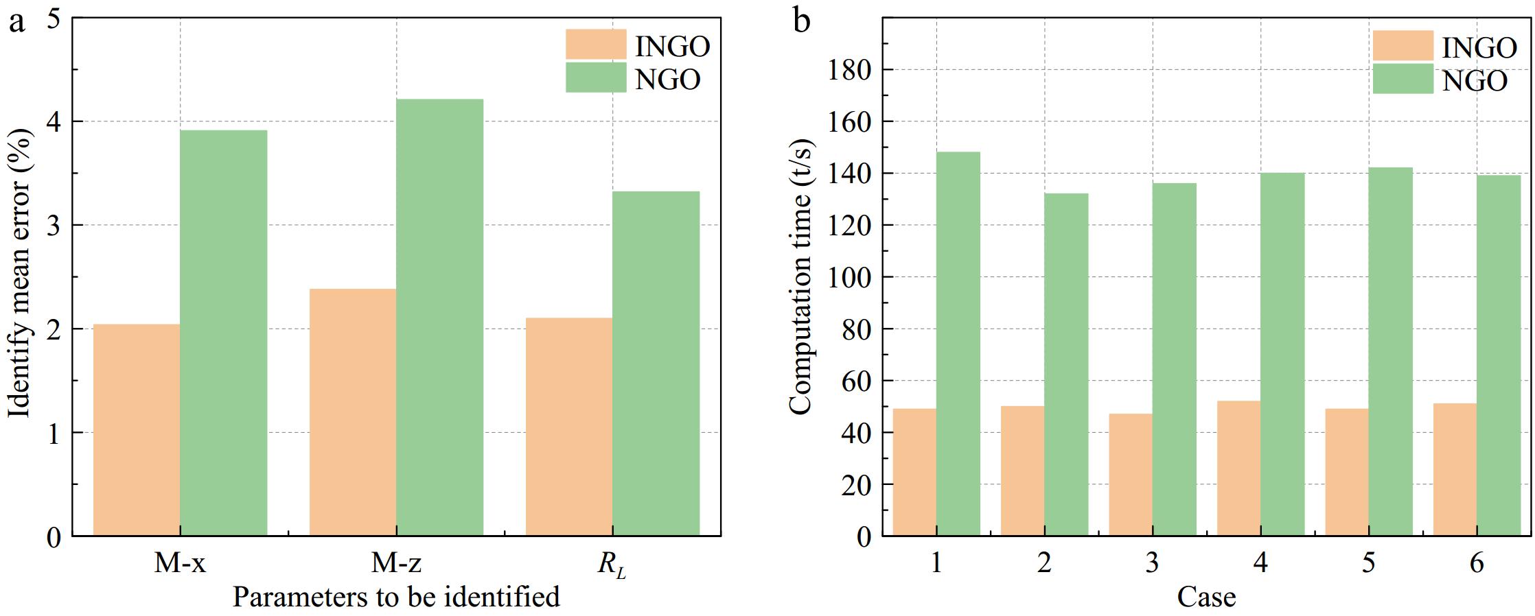
Figure 12.
Comparison of INGO and NGO algorithms. (a) Comparison of average error. (b) Comparison of computing time.
After applying the proposed scheme, the optimal equivalent load at the current level of offset can be calculated by using the mutual inductance parameters obtained from the algorithm identification using Eqn (6). Figure 13 illustrates the relationship between the optimal equivalent load corresponding to when the coil is horizontally offset and the actual load of the system. By adjusting the duty cycle of the switching tube of the Sepic circuit, the current equivalent resistance is transformed into the optimal equivalent resistance value, which can achieve the maximum efficiency of the system transmission. The duty cycle can also be calculated by Eqn (16) when the system load is changed to achieve maximum efficiency. Figure 14 shows the comparison of the system transmission efficiency when the coil level is offset and when the load is changed with or without using the impedance matching circuit, from which it can be seen that the system always works at maximum efficiency after using the impedance matching circuit, which verifies the effectiveness of the Sepic impedance converter.
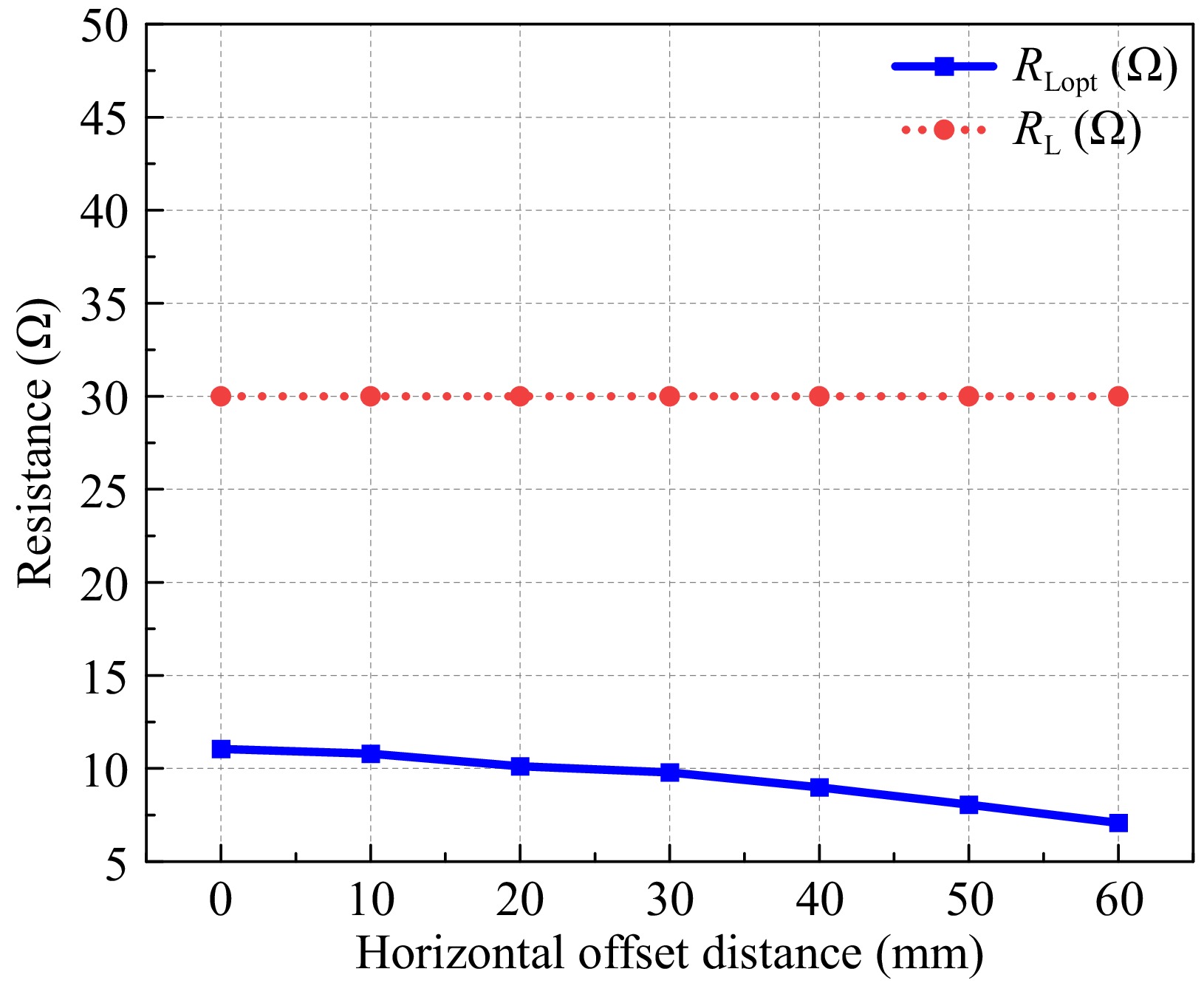
Figure 13.
Equivalent resistance calculated from recognised mutual inductance.
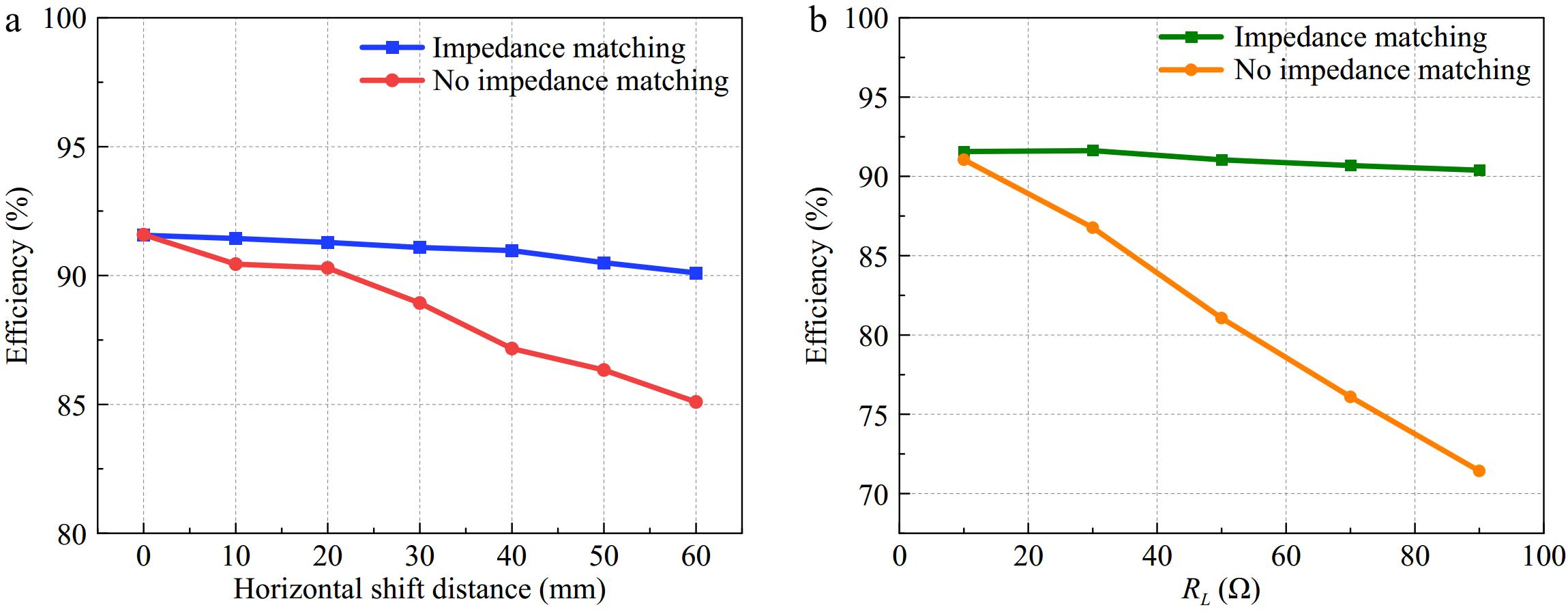
Figure 14.
Transmission efficiency with or without impedance matching applied (a) coil shift, (b) load variation.
$ {U_{{\text{out}}}} = \dfrac{{{N_1} + {N_2}}}{{{N_1} + 3{N_2}}}{U_{dc}} $ (22) The relationship between the output voltage and the input voltage of the system modulated by the pulse frequency is given by Eqn (22), and the different output voltages required by the load can be satisfied by adjusting the values of N1 and N2. At this time the system operating frequency is[26]:
$ {f_{PFM}} = \dfrac{{{N_1} + {N_2}}}{{{N_1} + 3{N_2}}}f $ (23) From Eqn (23), it can be seen that the switching frequency can be effectively reduced by the PFM system. The switch can be effectively turned on/off before the current crosses the zero point to achieve soft switching. Figure 15 illustrates the comparison of system transmission efficiency when two different modulation strategies are applied.
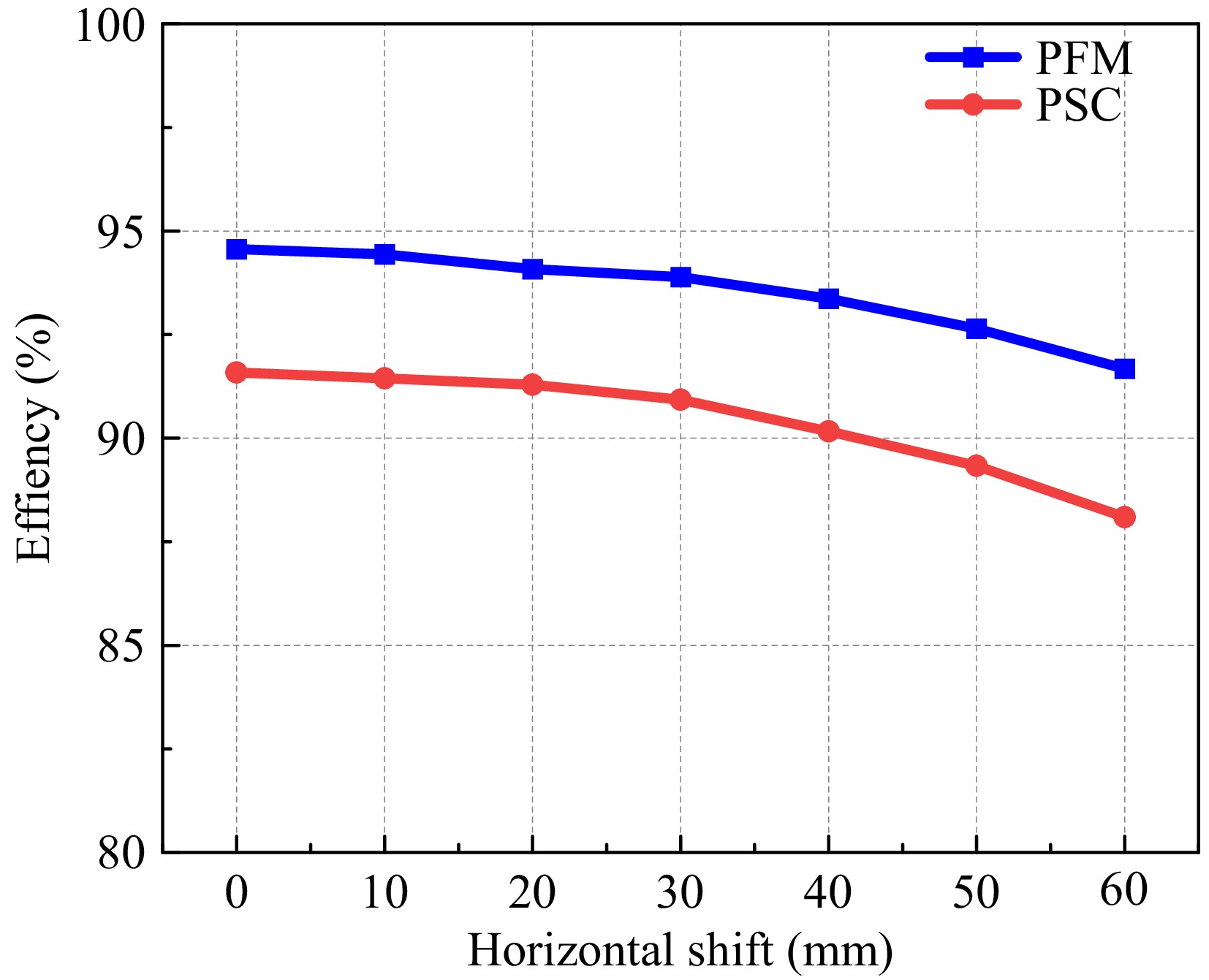
Figure 15.
Comparison of efficiency at different control strategies.
To highlight the differences between the method proposed in this paper and other tuning methods, Table 7 presents a comparative analysis of several features. Compared with other research strategies, this approach simplifies the control method, reduces the identification complexity, and minimizes the circuit size[16,17,27]. In comparison with the study by Guo et al.[19], although the identification complexity is similar, the method proposed here achieves higher identification accuracy. Therefore, a comprehensive comparison demonstrates the superiority of the proposed method, which can also be easily adapted to different topologies by modifying the mathematical model in the algorithm.
Table 7. Compared with other identification methods.
-
The experimental results validate the effectiveness of the proposed method in achieving high-precision parameter identification and maximum efficiency tracking. Compared to existing approaches, our work offers several key advancements. First, traditional methods such as those reported by Liu et al.[16] and Yang et al.[17] rely on additional circuits or complex switching operations, which increase hardware complexity and cost. In contrast, our method simplifies the system design by requiring only transmitter-side current measurements, eliminating the need for extra components. Second, the proposed INGO algorithm addresses the limitations of conventional optimization techniques by integrating an optimal value guidance strategy, a subtraction optimizer, and Cauchy mutation. These improvements enhance global convergence speed and reduce identification errors, making it particularly suitable for dynamic scenarios like EV charging where real-time adaptability is critical.
Furthermore, the PFM strategy adopted in this work overcomes the drawbacks of traditional modulation methods like PSC (high switching losses) and PDM (output fluctuations), achieving stable performance with reduced control complexity. Combined with the Sepic impedance matching circuit, our method ensures maximum efficiency tracking even under load variations and coil misalignment, as demonstrated in Fig. 14. Experimental results across diverse conditions—including horizontal/vertical offsets and load changes—confirm that the identification error remains below 3.5%, highlighting its robustness in practical applications.
While the current study focuses on SS-type topology, future work will extend this methodology to more complex topologies (e.g., LCC-LCC) and investigate environmental impacts (e.g., temperature) to broaden its applicability.
-
In this paper, a parameter identification method based on the INGO is proposed to achieve accurate identification of mutual inductance and loads between coils with lateral as well as longitudinal offsets, and by tracking the maximum efficiency of the WPT system through the identified parameters. Compared with other identification methods, algorithm identification has the advantages of reducing circuit complexity. Finally, the effectiveness of the proposed method is verified through experiments, and the experimental results show that the error of parameter identification can be kept within 3.5% by the method proposed in this paper, and the efficiency is effectively improved by the method of impedance matching.
This work was partially supported by the Natural Science Foundation of Shandong Province (Grant No. ZR2022ME214).
-
The authors confirm contribution to the paper as follow: study conception and design: Guo Z, Chen S; data acquisition and data collation: Guo Z, Chen S, Zhang H, Li Z, Yu H; analysis of simulation results: Guo Z, Chen S, Nai J, Ye M; writing manuscript review & editing: Guo Z, Chen S, Tian Y; access to funds: Zhang M. All authors have read and agreed to the final version of the manuscript.
-
All data generated or analyzed during this study are included in this published article.
-
The authors declare that they have no conflict of interest.
- Copyright: © 2025 by the author(s). Published by Maximum Academic Press, Fayetteville, GA. This article is an open access article distributed under Creative Commons Attribution License (CC BY 4.0), visit https://creativecommons.org/licenses/by/4.0/.
-
About this article
Cite this article
Guo Z, Chen S, Ye M, Nai J, Yu H, et al. 2025. Parameter identification method for a wireless power transfer system based on the Improved Northern Goshawk Optimization Algorithm. Wireless Power Transfer 12: e011 doi: 10.48130/wpt-0025-0007 

Parameter identification method for a wireless power transfer system based on the Improved Northern Goshawk Optimization Algorithm
- Received: 24 December 2024
- Revised: 19 February 2025
- Accepted: 07 March 2025
- Published online: 08 May 2025
Abstract: This paper proposes a mutual inductance and load parameter identification method using an Improved Northern Goshawk Optimization (INGO) Algorithm after pulse frequency modulation (PFM), and validates the effectiveness of the proposed parameter identification method through a maximum efficiency tracking approach. One of the most challenging aspects of wireless power transfer (WPT) technology for electric vehicles is the variation in the magnetic coupling coefficient between the two coils due to inaccurate parking positions and differences in height. First, a steady-state circuit model of an SS-type compensation network and pulse frequency modulation strategy was established to determine the correlation between system parameters. The INGO was then introduced to convert the parameter identification problem into an optimization problem, enabling the identification of load and mutual inductance parameters. Finally, the proposed identification method was experimentally validated, and the maximum efficiency tracking of the proposed WPT system was achieved through a Sepic impedance matching circuit. The results show that the identification method can maintain high accuracy even under coil displacement and load variation conditions.