The recognition of wire icing risk levels based on deep learning

Wire icing refers to the phenomenon of wet snow freezing on wires or the adhesion of rime or glaze ice on wires^[1]. Wire icing can cause incidents such as cable galloping and breakage, tower collapse, and insulator flashover^[2]. From January to February 2008, four severe freezing rain and snow events occurred consecutively in southern China, resulting in significant damage to power, transportation, and other sectors^[3]. Research on wire icing in China began relatively late, with the first wire icing observation station established in late 1964 at Bailong Mountain in Huidong County, Sichuan Province^[4]. Since then, numerous scholars have conducted a series of studies using observational data from meteorological and power system departments to explore the weather and climatic characteristics of wire icing events^[5−7], the microphysical mechanisms of formation^[8,9], and the simulation of icing processes^[10−12].

Conventional wire icing observation methods rely mainly on manual observations, which are time-consuming and labor-intensive, making it difficult to obtain continuous data on icing dynamics and limiting the capability to monitor wire icing risks. The successful development of automated wire icing monitoring equipment has effectively addressed some of the limitations of manual observations. This equipment uses weight sensors mounted at both ends of the wire to measure the deformation caused by ice accumulation, converting these measurements into electrical signals that are transmitted to a data acquisition and processing unit, which calculates the corresponding weight. This system can automatically monitor and record the continuous changes in icing weight with a time resolution as high as once every 10 s^[13]. However, the high cost of this equipment makes it challenging to deploy on a large scale for routine observation operations.

Some empirical models used in wire icing have simple structures and easily accessible parameters but perform poorly^[14]. Additionally, some numerical models are limited by the difficulty of parameterizing wire icing from freezing rain and wet snow, making them applicable only to rime wire icing^[15,16]. Although some domestic scholars have improved these empirical models based on local climate conditions and achieved satisfactory simulation results, the improved models are not applicable to other regions^[17−19]. Some researchers have also used multiple linear regression or stepwise linear regression to construct linear models between ice thickness (or standard ice thickness) and meteorological factors for simulation^[20,21]. However, since wire icing is a complex nonlinear process, the results obtained through linear regression methods fail to meet practical requirements. This demonstrates that simulating wire icing remains a highly challenging problem.

In recent years, Convolutional Neural Networks (CNN) have been widely used in the fields of image classification, object detection, and image recognition due to their simple network architecture and powerful feature extraction and classification capabilities^[22]. Palvanov & Cho^[23] employed a multi-branch CNN to identify fog levels, while Han et al.^[24] used a deep convolutional residual neural network (ResNet) to develop a machine learning-based parameterization model that provided temperature tendencies, water vapor tendencies, and information on cloud water and cloud ice due to non-adiabatic processes in cumulus clouds. Additionally, Zhou et al.^[25] applied an improved VGG16 model for the similarity recognition and application evaluation of the subtropical high-pressure system, achieving favorable results in these studies. Therefore, utilizing images of wire icing as a supplementary tool for risk monitoring offers a promising alternative. This study aims to identify a model with high recognition efficiency and strong transfer learning capabilities to classify images of wire icing and assess its risk levels, thereby providing a new method for wire icing risk level identification.

This study selected two commonly used models in image recognition, VGG16, and ResNet34, as the base convolutional neural network models. The wire icing images were fed into the convolutional neural networks, which then processed the images to output their corresponding categories. VGG16, as one of the best-performing models in the VGGNet (Visual Geometry Group Network), achieved second place in the ImageNet Large Scale Visual Recognition Challenge (ILSVRC) classification task in 2014^[26]. It comprises 13 convolutional layers and three fully connected layers, with all convolutional layers using 3 × 3 kernels^[27]. This design helps increase the network's non-linear representation capability and reduces the number of parameters. Max-pooling layers are used between the convolutional layers to down-sample the feature maps, aiding in the extraction of more abstract and higher-level features. Following the convolutional section are three fully connected layers that map the extracted features to category scores. ResNet (Residual Networks), a deep residual network proposed by Microsoft Research Asia in 2015, addresses issues like gradient vanishing and network degradation caused by increasing network depth by introducing residual structures^[28]. ResNet34, as a significant member of the ResNet family, has a simple architecture, fast computation speed, and outstanding performance. It contains 32 residual blocks, with the first 16 residual blocks comprising eight basic convolutional layers, and the latter 16 residual blocks comprising 16 basic convolutional layers. This structure enables the network to efficiently extract image features, yielding excellent performance in image classification tasks.

Loss function selection

The loss function is used in deep learning to measure the difference between the predicted outputs of a model and the actual labels^[29]. This study adopted the Cross-Entropy Loss Function (CELF). In image recognition, the CELF is widely used, originating from information theory, and is used to describe the difference in probability distributions between random variables or a set of events^[30]. In pixel-level image classification tasks, the CELF has demonstrated good performance. Its curve is convex and generally monotonic, with an increasing gradient as the loss increases, providing a more rapid optimization path for backpropagation. The relationship is represented by Eqn (1):

where, y_i represents the i-th element of the actual probability distribution, and p_i represents the i-th element of the predicted probability distribution.

Model optimization

During the model training process, the optimal learning rate was determined by using the cross-entropy loss function and classification accuracy as evaluation criteria. The performance of the VGG16 and ResNet34 models was compared to select the better-performing model for optimization. The specific optimization strategies were as follows: Normalization and dropout algorithms were applied to the image pixels before training to reduce overfitting^[31,32]. Additionally, data augmentation techniques such as random horizontal and vertical flipping and random color enhancement were employed to improve the model's generalization capability. A transfer learning approach, based on fine-tuning pre-trained weight parameters, was adopted to accelerate model convergence and enhance accuracy while ensuring that global parameters remained adjustable for the best model performance. The specific values of the adjusted hyperparameters or the optimization algorithms are detailed in Table 1 and the specific experimental process of this study are shown in Fig 1.

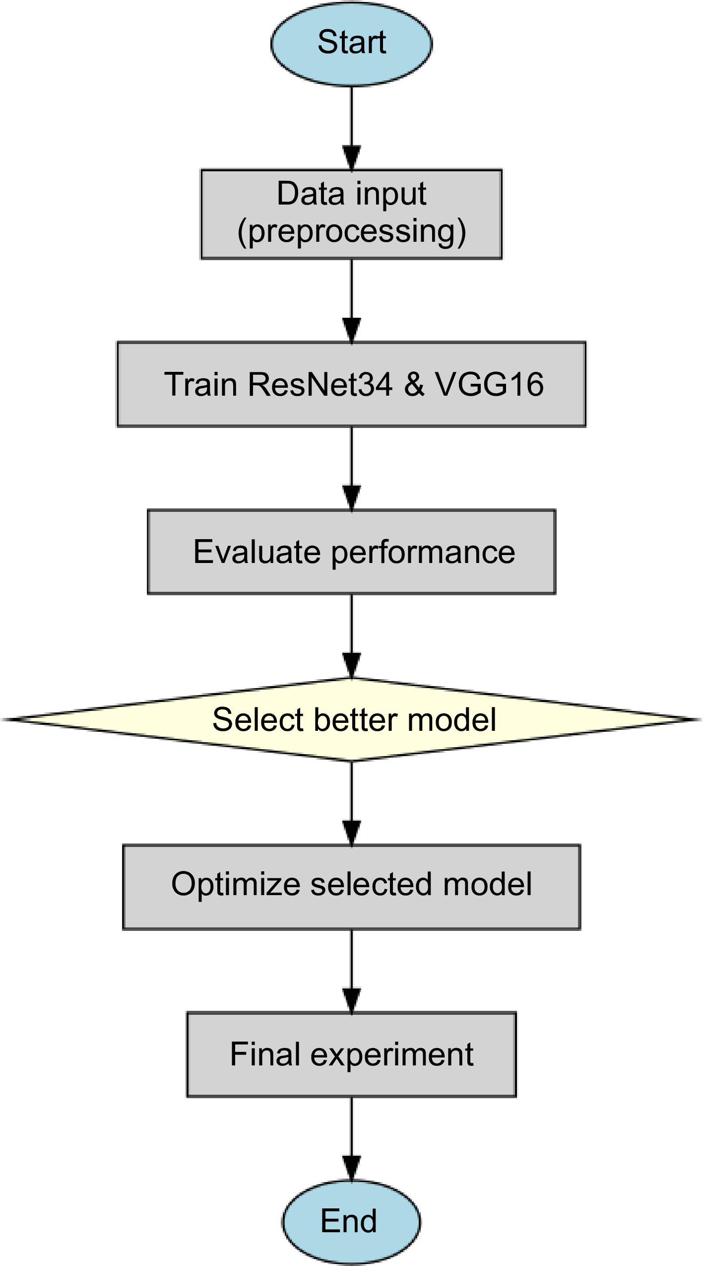
Figure 1. 

Experimental procedure.

Observation site 1 is located at the Enshi Weather Radar Station in Hubei Province, China (30.28° N, 109.27° E, elevation 1,722 m a.s.l.), with observation data collected during the winter seasons from 2019 to 2021. Observation site 2 is situated at Shennongding in the Shennongjia region of Hubei Province (31.45° N, 110.31° E, elevation 3,105.4 m a.s.l.), with data collected from December 2019 to January 2020. Observation site 3 is at the Lushan Meteorological Bureau Observation Site in Jiangxi Province (29.58° N, 115.98° E, elevation 1,164.5 m a.s.l.), with observation data gathered from December 2016 to February 2017. The geographical locations of these three observation points are shown in Fig 2. Each of these observation points features unique mountainous climatic characteristics and complex terrain, with ample moisture supply. The convergence of warm and cold air masses during the winter often leads to the formation of various forms of precipitation, including freezing rain, supercooled fog, and snow^[8,9,33]. Therefore, they are ideal sites for observing wire icing phenomena.

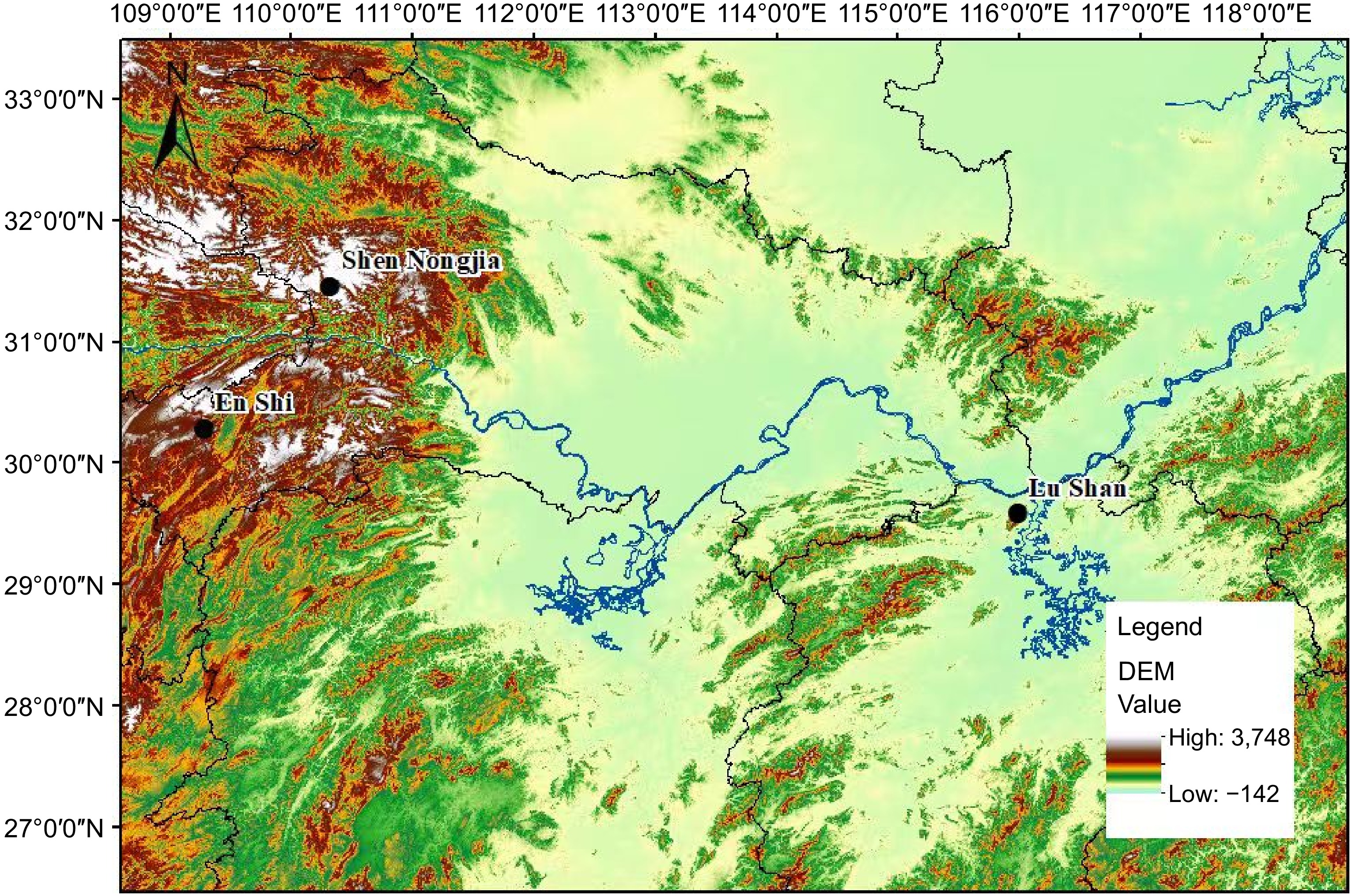
Figure 2. 

Geolocation of the observation sites.

Observation instruments

The observation instrument used for wire icing is the NH3000 automatic wire icing monitoring system, as shown in Fig 3. The setup consists of two wire icing frames oriented in the east-west and north-south directions, with a distance of 1.5 m between them. Each frame holds a steel-core aluminum wire that is 100 cm in length and 26.8 mm in diameter, as specified by the 'Surface Meteorological Observation Specifications: Wire Icing' standards^[1]. Each wire icing frame is connected to an ice-weight sensor, which can automatically measure and record the continuous changes in wire icing weight, with measurements taken every minute. Additionally, a camera is mounted above each wire icing frame to record video and capture images of the icing process, providing a more accurate and objective representation of the continuous changes during a single icing event, with images captured every 15 min. The ice weight data and wire icing images are collected simultaneously, and the system is equipped with a wireless transceiver function for real-time remote data transmission.

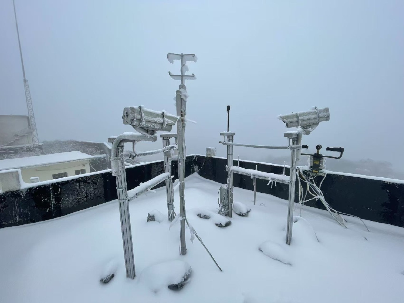
Figure 3. 

The NH3000 automatic wire icing monitoring system and its installation setup.

Wire icing image data

According to the 'Meteorological Industry Standards of the People's Republic of China' issued by the China Meteorological Administration^[34], the risk levels of wire icing are classified into four categories based on the standard ice thickness (B₀). These categories are as follows: Level 1 (light): B₀ < 5 mm; Level 2 (moderate): 5 mm ≤ B₀ < 10 mm; Level 3 (heavy): 10 mm ≤ B₀ < 15 mm; and Level 4 (severe): B₀ ≥ 15 mm. The standard ice thickness is calculated using Eqn (2). Based on this, the risk levels defined by standard ice thickness can be converted to risk levels based on ice weight (w) as follows: Level 1 (light): 0 < w < 450 g; Level 2 (moderate): 450 g ≤ w < 1,040 g; Level 3 (heavy): 1,040 g ≤ w < 1,770 g; and Level 4 (severe): w ≥ 1,770 g.

Equation (2) defines B₀​ as the standard ice thickness (mm), w as the wire icing mass (g, rounded to the nearest integer), L as the wire length (m), and r as the wire radius (in mm). Considering that some images were captured when no wire icing was present or had already dissipated, we added an additional level: Level 0 represents the absence of icing. Since the imaging equipment was not equipped with a flash, night-time wire icing images could not be obtained, and the data used in this study were limited to the period between 6:00 and 19:00.

In this study, we selected wire icing images from Enshi and Shennongjia to compare the performance of the VGG16 and ResNet34 models, while the wire icing images from Lushan were used to test the optimized model's recognition ability in different regions. Initially, we performed quality control on the images, discarding those where the lens was covered with ice or snow, or where lighting was insufficient. After quality control, a total of 9,483 wire icing images were available from the two sets of wire icing monitoring systems in Enshi and Shennongjia. The data distribution across the categories is imbalanced, with 4,146 images in Level 1 (light), accounting for 43.7% of the total, while only 92 images belong to Level 4 (severe), comprising just 9.7% of the total. Such imbalanced data distribution can cause the model to favor classes with more samples during training, resulting in instability and lower recognition accuracy^[35]. Furthermore, factors like wind speed and direction cause the distribution of wire icing on the wires to be uneven^[36], meaning that standard ice thickness does not fully capture the true state of wire icing. Taking these factors into account, we adjusted the classification levels for ice weight as follows: Level 0 (no icing) w = 0, Level 1 (light) 0 < w < 200 g, Level 2 (moderate) 200 g ≤ w < 450 g, Level 3 (heavy) 450 g ≤ w < 1,040 g, and Level 4 (severe) w ≥ 1,040 g. After this reclassification, the data balance improved significantly, the data includes 2,884, 2,865, 1,281, 1,713, and 740 images classified as Level 0, Level 1, Level 2, Level 3, and Level 4, respectively.

Image preprocessing

Considering that the camera placement at each observation point is fixed, to enhance the model's generalization capability, we performed batch cropping on the original images, retaining only a segment of the wire. This approach maximally reduces the interference of background factors on the model training. The cropping size was set to 128 × 256 pixels. The original images and the cropped images of different wire icing risk levels are shown in Fig 4.

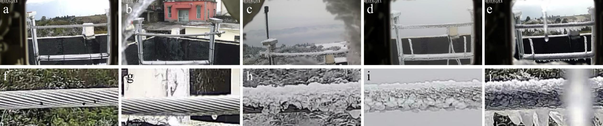
Figure 4. 

(a)−(e) Original and (f)−(j) cropped images of wire icing for different risk levels (Levels 0−4).

Experimental environment and parameters

The experiments were conducted on a Windows 11 operating system, with the machine configured as follows: CPU: Intel Core i5-13400F, 4.60 GHz; GPU: GeForce GTX 3060, 12GB. The experiments utilized the pytorch deep learning framework, and the programming language used was Python. The training of the network was carried out using the Stochastic Gradient Descent (SGD) method.

The training set, validation set, and test set were divided according to the commonly used ratio of 7:1:2. A total of 6,637 images were randomly selected from Enshi and Shennongjia as the training set for model input, with 948 images used as the validation set for adjusting the model's hyperparameters during training, and 1,898 images as the test set for the final model evaluation.

We first compared the cross-entropy loss function curves and accuracy curves of the training and validation sets for the VGG16 and ResNet34 models, as shown in Fig 5. It can be observed that the cross-entropy loss on the training and validation sets for the ResNet34 model is lower than that of the VGG16 model. Moreover, the recognition accuracy of the ResNet34 model on both the training and validation sets is superior to that of the VGG16 model. This is attributed to the fact that, compared to the shallower VGG models, the residual structure of ResNet34 allows for increased network depth while maintaining gradient stability. The residual block, as a robust and fault-tolerant basic structure, enables the original signal to be directly transmitted to the deeper layers of the network through nonlinear mapping, thus avoiding issues like gradient explosion and vanishing gradients that may occur during backpropagation. In contrast to the potential distortion and gradient instability in the deeper layers of VGG, the residual blocks reduce the computational complexity of the network while preserving performance, demonstrating excellent adaptability and robustness^[37,38].

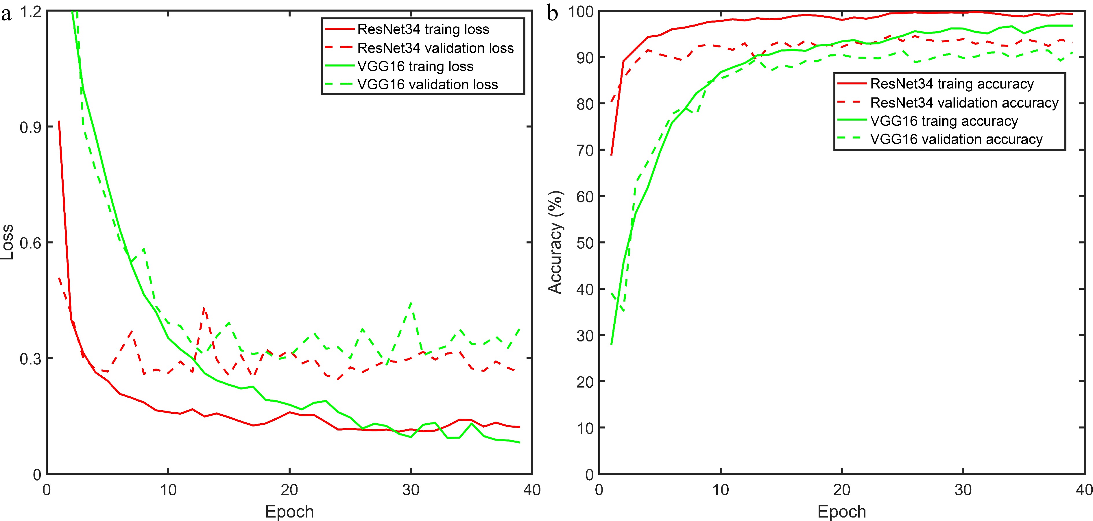
Figure 5. 

(a) Cross-Entropy Loss curves and (b) accuracy curves for the training and validation sets of VGG16 and ResNet34 models.

Although the ResNet34 model generally exhibits stronger recognition capabilities for wire icing risk levels compared to VGG16, it still faces similar issues, with a significant difference of about 0.2 between the cross-entropy losses of the training and validation sets, and the training set accuracy being over 5% higher than that of the validation set. This indicates that the model is experiencing overfitting, meaning it has become too closely aligned to the training data and has lost its generalization ability for unseen data. An overfitted model may perform poorly on new data that was not present in the training set, leading to issues in practical applications when faced with diverse data^[39]. Therefore, we optimized the ResNet34 model using the method described previously. The cross-entropy loss function curves and recognition accuracy curves for the ResNet34 model and the optimized ResNet34 model (ResNet34+) are shown in Fig 6. It is evident that the cross-entropy loss for the validation set of the ResNet34+ model have significantly decreased, and the difference between the training and validation sets has reduced. Similarly, while the validation accuracy of the ResNet34+ model remained almost unchanged compared to that of the ResNet34 model, the validation accuracy of the ResNet34+ model showed a marked improvement over ResNet34, and the gap between the training and validation accuracies has significantly decreased. This indicates that the generalization ability of the ResNet34+ model has improved notably compared to that of the ResNet34 model, and the ResNet34+ model achieves a good recognition accuracy for wire icing risk levels.

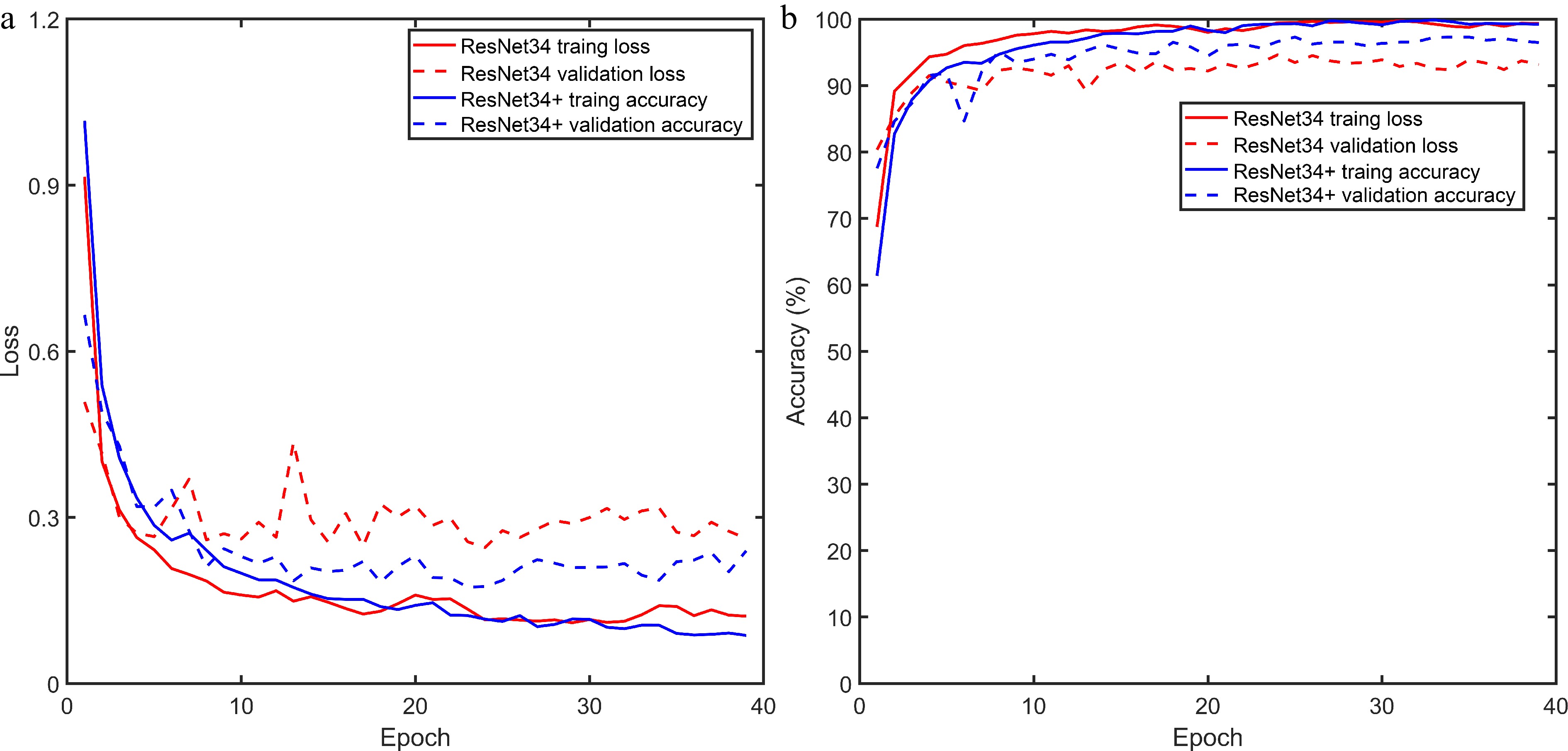
Figure 6. 

(a) Cross-Entropy Loss curves and (b) accuracy curves for the training and validation sets of ResNet34 and ResNet34+ models.

The use of the confusion matrix method allows for a visual evaluation of the performance of the wire icing risk level recognition models. When the output risk level of wire icing from the model matches the actual risk level, it is considered an accurate sample. The confusion matrices for the recognition accuracy of the ResNet34 and ResNet34+ models on the test set are shown in Fig 6. From Fig. 7, it can be observed that the recognition accuracies of the ResNet34+ model for the five levels of wire icing risk are 94.5%, 91.2%, 89.6%, 96.3%, and 96.7%, respectively, indicating that the ResNet34+ model outperforms the ResNet34 model across all risk levels.

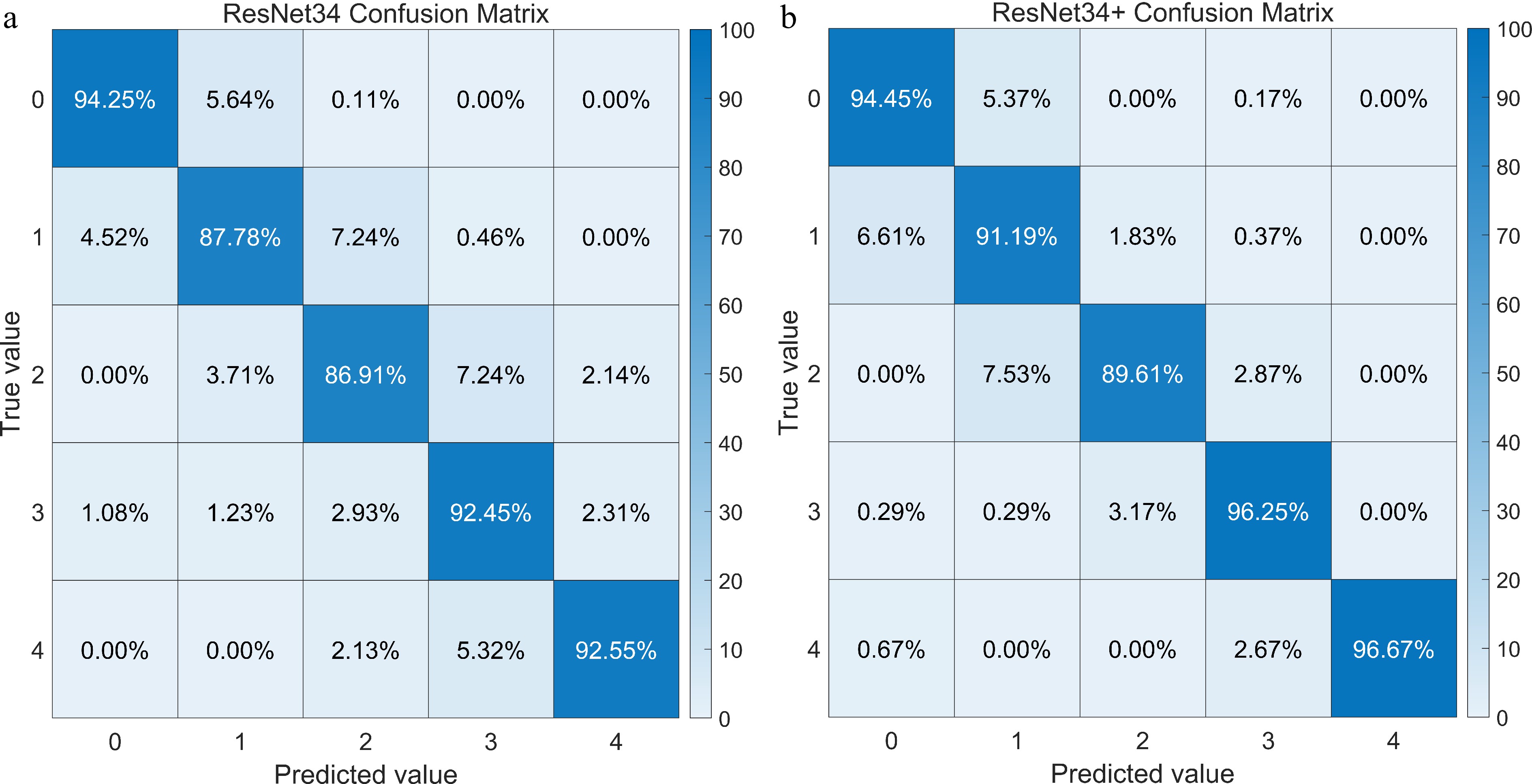
Figure 7. 

Confusion matrix of the recognition accuracy for different wire icing risk levels using the (a) ResNet34 and (b) ResNet34+ model.

However, the recognition accuracies of the ResNet34+ model for levels 1 and 2 are slightly lower than those for the other three levels. This is attributed to the fact that, in the case of light risk, the amount of wire icing is minimal, resulting in a small difference between the images with light icing and those with no icing. Consequently, 6.61% of the light icing instances were misclassified as no icing. Similarly, the distinguishing features between the images of light icing and moderate icing are not very pronounced, leading to 7.53% of moderate icing instances being misclassified as light icing.

To assess the recognition performance of the ResNet34+ model on wire icing risk levels across different regions and directions of wires, the confusion matrix for the model's recognition accuracy on wires in various locations and orientations is presented in Fig 8. It can be seen that, aside from the subpar recognition performance in the Shennongjia region due to the limited sample sizes of moderate, heavy, and severe risk levels—where there were only 32, six, and five samples, respectively— the recognition accuracies for all other risk levels exceeded 83%. This indicates that the ResNet34+ model demonstrates good generalization performance.

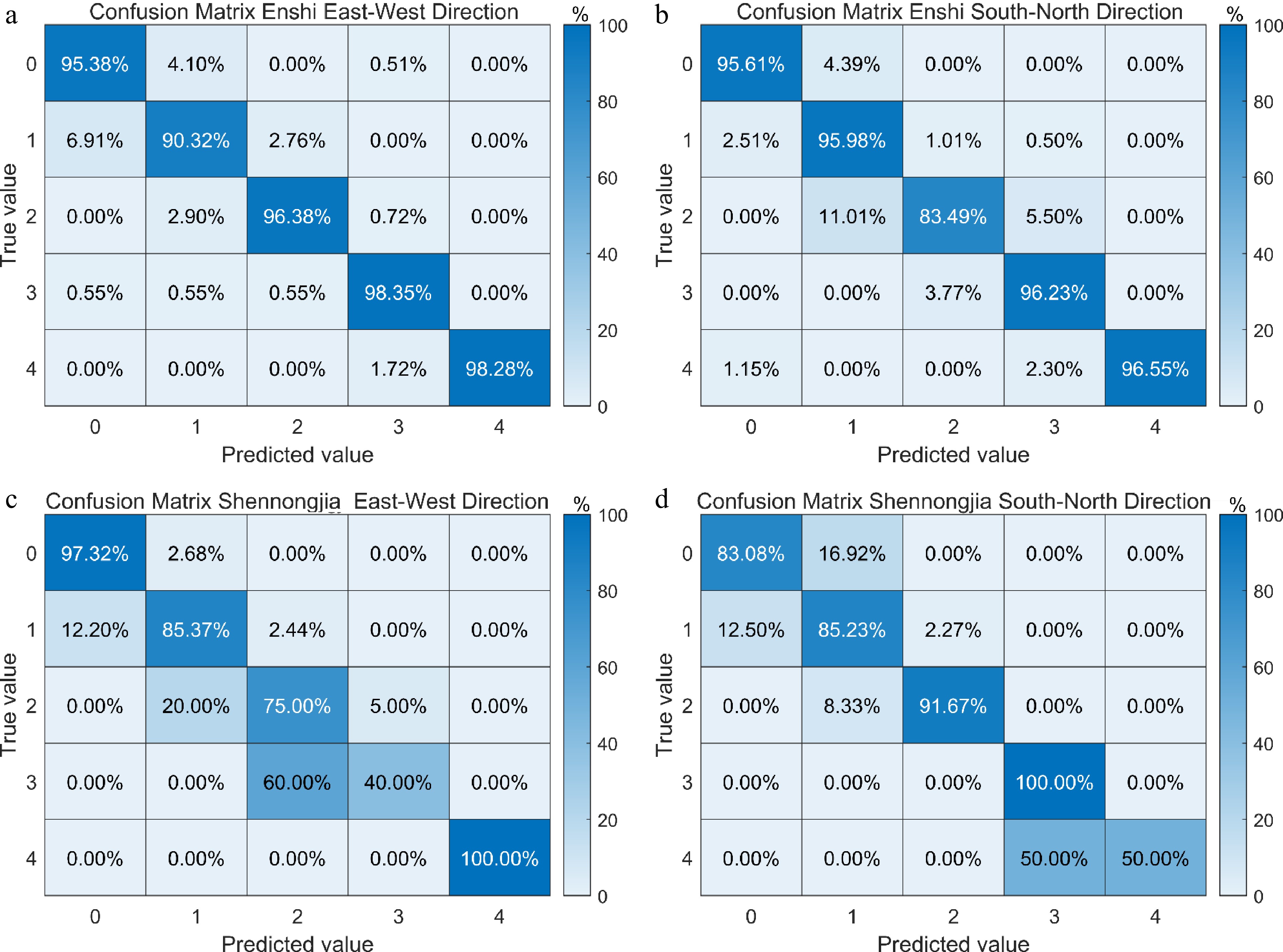
Figure 8. 

Confusion matrices of the recognition accuracy for different wire icing risk levels using the ResNet34+ model in various regions and different directions of wires: (a) Enshi East-West direction, (b) Enshi North-South direction, (c) Shennongjia East-West direction, and (d) Shennongjia North-South direction.

Figure 9 illustrates the variation in the recognition accuracy of the ResNet34+ model for wire icing risk levels across different time periods. The average recognition accuracy for wire icing risk levels during these periods reached 93.3%. The time frames with higher accuracy were between 08:00 to 11:00 and 15:00 to 17:00 Beijing time. This improvement in accuracy can be attributed to favorable lighting conditions during these hours, which resulted in clearer images and more distinct features of wire icing, achieving an average recognition accuracy of 94.7%. In contrast, during the early morning and evening hours, the lower light conditions led to image blurriness, resulting in lower average recognition accuracies of only 91.4% between 06:00 to 07:00 and 18:00 to 19:00. Additionally, between 12:00 and 14:00, the strong lighting conditions caused image overexposure, leading to a loss of details in the images; consequently, the average recognition accuracy during this period was also relatively low, at 90.9%.

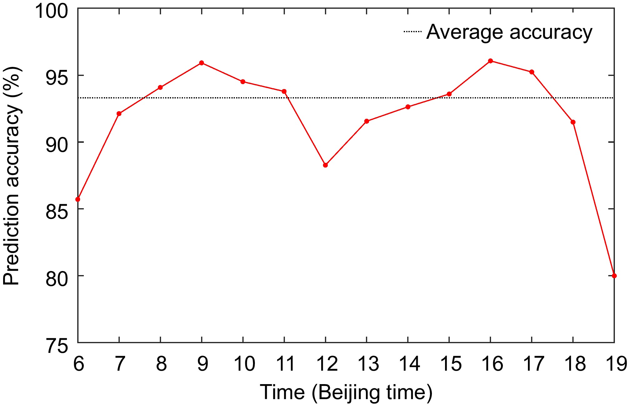
Figure 9. 

The accuracy curves for different time intervals in wire icing risk level identification.

To evaluate the stability of the ResNet34+ model in different regions, we inputted 230 images from both east-west and north-south oriented wires, collected during a rain-fog mixed wire icing event at Lushan from January 10 to 13, 2016, into the ResNet34+ model. The confusion matrices for recognition accuracy in both orientations, along with the recognition accuracy variation curves for wire icing risk levels across different time periods, are shown in Fig 10. Although the foggy conditions resulted in less clear images, the ResNet34+ model still demonstrated good applicability in the Lushan region, achieving an average recognition accuracy of 89.4% for the east-west orientation and 90.8% for the north-south orientation. The model showed the highest recognition accuracy for no icing in the east-west orientation, while it excelled in recognizing severe wire icing in the north-south orientation. The recognition accuracy for the east-west orientation was relatively high from 10:00 to 16:00, whereas the north-south orientation exhibited higher accuracy during the periods of 11:00 to 13:00 and 15:00 to 17:00.

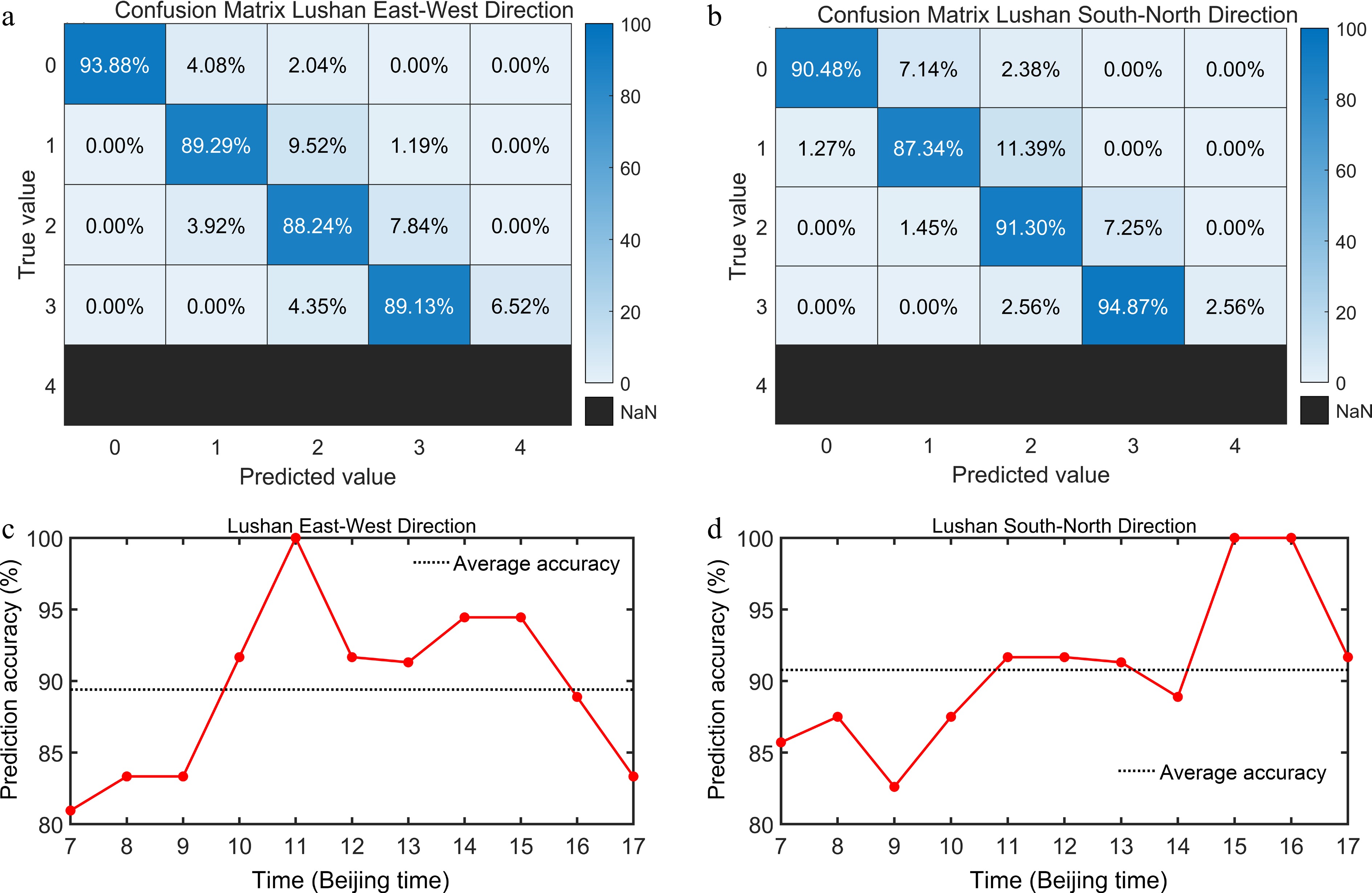
Figure 10. 

Confusion matrices of the recognition accuracy for different wire icing risk levels using the ResNet34+ model in different directions of wires (a), (b) and the accuracy curves for different time intervals in ice accumulation risk level identification (c), (d) in Mount. Lu.

Wire icing can cause significant economic losses, yet existing observation methods have limited capacity to identify wire icing risk levels. This study aims to recognize wire icing risk levels by inputting images of wire icing into deep learning models. The results indicate:

The ResNet34 model outperforms the VGG16 model in identifying wire icing risk levels. The optimized ResNet34 model (ResNet34+) which incorporates normalization processing, dropout algorithms, and data augmentation techniques, demonstrates good performance in recognizing wire icing risk levels for wires in different regions and orientations, achieving an overall recognition accuracy of 93.3%. The periods with higher accuracy occur between 08:00 and 11:00 and 15:00 and 17:00 Beijing time.

The ResNet34+ model shows good recognition performance for wire icing risk levels in both east-west and north-south orientations during a rain-fog mixed wire icing event in Lushan, with average recognition accuracies reaching 89.4% and 90.8%, respectively. This indicates that the ResNet34+ model has strong generalizability and can provide a novel approach for recognizing wire icing risk levels.

Our method is designed to classify the icing risk level with high accuracy, rather than to predict the exact ice thickness on wires. While it cannot replace direct observation, it provides an effective tool for early warning and risk assessment in power grid operations. The primary application value of our work lies in its potential to enhance decision-making processes for grid maintenance and disaster prevention, allowing operators to take timely protective measures. However, due to the limited number of image samples collected in this study, we still need to enhance the model's applicability by increasing the training data and employing transfer learning. Additionally, constrained by the image capture equipment, this study could only recognize wire icing risk levels during the daytime. In future research, we plan to improve the image capture devices to enable the collection of clear wire icing images at night, thus facilitating round-the-clock identification of wire icing risk levels.