Constant voltage output disturbance rejection control for WPT systems applied to offshore floating platforms

Wireless power transfer (WPT) systems have been widely adopted in fields such as electric vehicles, biomedical engineering, portable devices, and unmanned aerial vehicles^[1−4] due to their high safety, reliability, and flexibility.

In magnetic-coupled WPT systems for marine engineering, two primary application scenarios exist: surface and undersea systems. Undersea applications focus on addressing energy supply challenges for underwater equipment, while surface applications involve WPT between shore and ships, or between ships^[5,6]. Notably, both scenarios suffer from coil misalignment and power transmission fluctuations due to ocean currents and waves.

Current strategies for suppressing power fluctuations fall into three categories: the couplers design with high misalignment tolerance^[7], the development of hybrid compensation topologies^[8], and the implementation of system-level control strategies^[9]. This paper addresses WPT between networks of offshore floating platforms with marine energy harvesting capabilities. A strategy is proposed to suppress power fluctuations caused by time-varying mutual inductance by connecting the Buck converter in series at the receiver side, and controlling its duty cycle. The schematic diagram is illustrated in Fig. 1.

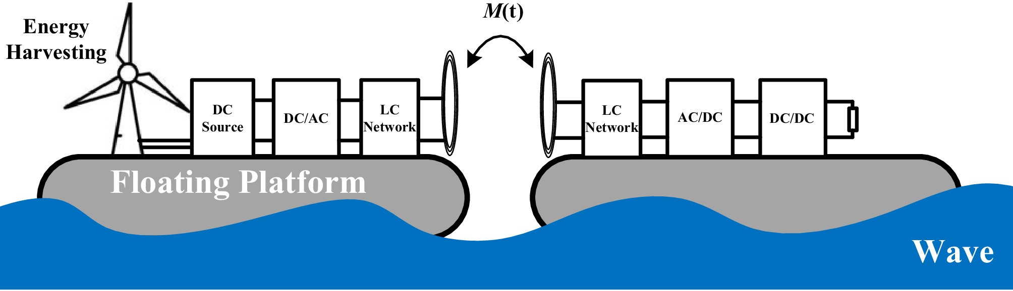
Figure 1. 

The schematic diagram of an offshore floating platform system with energy harvesting and WPT capabilities.

To obtain an accurate model of the Buck converter for enhanced control performance, conventional approaches rely on mechanism-based methods, including state-space averaging^[10] and small-signal modeling methods^[11]. However, these methods not only depend on precise circuit parameter measurements but are also limited to linearization around a static operating point, thus failing to capture the large-signal nonlinear behavior of the converter.

Therefore, this paper proposes a data-driven linear parameter-varying (LPV) modeling approach for the Buck converter to overcome the aforementioned limitations. The LPV model captures complex system dynamics through time-varying parameters, making it suitable for large-signal modeling of Buck converters with time-varying input voltages. Moreover, its inherently linear structure facilitates controller design and stability analysis using well-established linear theories. Additionally, the data-driven LPV modeling approach requires no parameter measurements, offering significant practicality and operational convenience.

To achieve constant-voltage output disturbance rejection control, a controller is designed for the LPV model. Model Predictive Control (MPC) is an online optimal control strategy based on precise models, which calculates the current control action by solving an optimization problem in real-time and performs receding horizon optimization. Numerous studies have applied MPC to WPT systems. An MPC algorithm with multi-step delay compensation was deployed for a dynamic wireless power transfer system^[12]. Also, MPC was used for power control and maximum efficiency tracking in bidirectional WPT systems^[13]. Meanwhile, MPC was employed for phase-shift control of the transmitter-side inverter in a WPT system^[14]. However, few studies have explored MPC for LPV model control. Moreover, MPC inherently accommodates time-varying models, making it suitable for LPV-based control.

This paper addresses a WPT system for offshore floating platforms with slowly varying mutual inductance, proposing an integrated modeling and control framework based on LPV open-loop identification and MPC. The main contributions are as follows:

(1) Utilizing the input voltage as the scheduling variable, the LPV model enables accurate large-signal modeling of the Buck converter.

(2) The data-driven LPV model parameter identification method requires no circuit measurements and offers strong operational practicality.

(3) Employing MPC to control the LPV model leverages its inherent capability to handle time-varying dynamics while maintaining straightforward parameter tuning.

The structure of the WPT system applied to the offshore floating platform, as constructed in this paper, is illustrated in Fig. 2. The transmitter side consists of a DC source V_dc, an inverter, and a series resonant topology (C_t, L_t). The receiver side includes not only a series resonant topology (C_r, L_r), a rectifier, a filter capacitor C_f, and a resistance R_L, but also an additional Buck converter connected in series to regulate the output voltage V_out. The parameters of the series resonant topologies satisfy the following relationship, where ω denotes the resonant frequency:

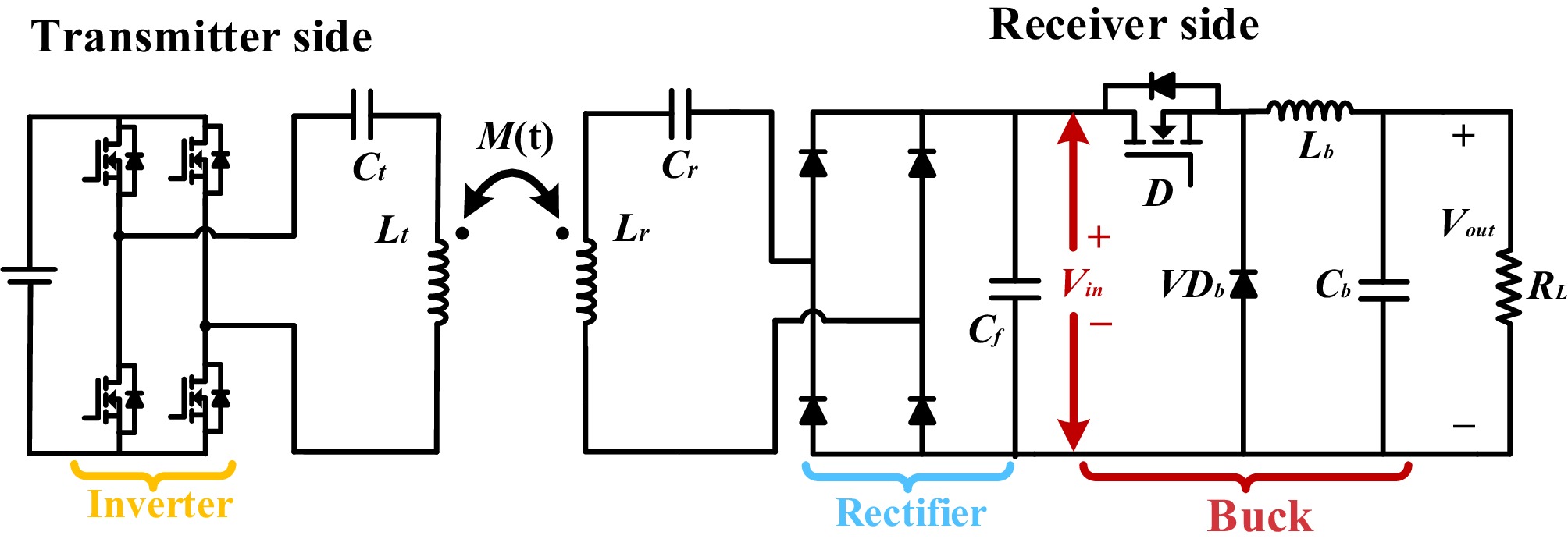
Figure 2. 

WPT System topology with Buck converter and time-varying mutual inductance.

Furthermore, due to the inevitable wave-induced motion of offshore floating platforms, when the transmitter and receiver of the WPT system are placed on two separate platforms for power transmission, the distance and angle between the transmitting (Tx) coil L_t and receiving (Rx) coil L_r will vary with platform motion. This introduces time-varying mutual inductance M(t) between them, ultimately leading to fluctuations in the Buck input voltage V_in and transmitted power.

This paper suppresses fluctuations of the output voltage V_out caused by time-varying mutual inductance M(t) by dynamically adjusting the pulse-width modulation (PWM) signal duty cycle D of the Buck, thereby achieving constant voltage output. Therefore, under constant switching frequency and continuous conduction mode (CCM), it is necessary to model the dynamic relationship of the Buck converter with the duty cycle variation ΔD as the input and the output voltage variation ΔV_out as the output.

Conventional linear modeling approaches for Buck converters, based on small-signal linearization around a static operating point, fail to capture the nonlinear characteristics under large-range operating point variations. To address this limitation, this paper introduces a linear parameter-varying (LPV) modeling methodology based on system identification for the Buck converter. The LPV model retains the simple structure of a linear model while incorporating scheduling variables, enabling it to characterize the dynamic behavior of time-varying systems. It is therefore well-suited for large-signal modeling of Buck converters.

LPV model structure

The standard form of a discrete-time single-input (i.e., duty ratio D) single-output (i.e., output voltage V_out) LPV model for the Buck converter can be expressed as:

At sampling time k, x(k) is the noise-free output, e(k) is the noise, and z⁻¹ is the backward shift operator. The input voltage V_in of the Buck converter serves as the scheduling variable that reflects the time-varying characteristics of the system, A and B are polynomials of orders n₁ and n₂ in z⁻¹, respectively, expressed as:

where, the coefficients a_i and b_j are dependent on the scheduling variable and can be commonly expressed as polynomial functions of V_in at sampling time k:

where, i = 1, 2, ···, n₁, j = 0, 1, ···, n₂, g_m (m = 1, 2, ···, n₃), and h_m (m = 1, 2, ···, n₄) are a priori chosen polynomials of V_in(k) with order n₃ and n₄. Therefore, the parameter vector $\boldsymbol{\theta } $ of the LPV model in Eq. (2) can be stacked as follows, which is obtained through subsequent parameter identification:

Parameter identification of the LPV model for the Buck converter

This paper employs the data-driven parameter identification approach to obtain the LPV model of Buck, as opposed to conventional mechanism-based modeling methods^[15,16]. Given that the Buck converter contains two energy storage elements (C_b, L_b), its model order is selected as 2, i.e., n₁ = 2. Furthermore, inspired by the commonly used small-signal model structure of the Buck converter^[17], the structure of the LPV model to be identified is selected a priori as follows:

with n₂ = 0, n₃ = 0, n₄ = 1, and

LPV model identification requires finding the parameter vector $\boldsymbol{\theta } $ to fit the sampled dataset D_S = {V_out(k), D(k), V_in(k)}, and minimize the mean square prediction error, where k = 1~N, N is the sampled data number.

Substituting Eq. (6) into Eq. (2) yields:

The one-step predicted error is minimized by the cost function L as:

where,

Eq. (10) can be derived as:

Dividing both sides of Eq. (11) by 1 + a₁,₀z⁻¹ + a₂,₀z⁻², and rewriting it in standard linear regression form yields:

The subscript A denotes dividing by A(V_in(k),z⁻¹) = 1 + a₁,₀z⁻¹ + a₂,₀z⁻².

The consistent and unbiased estimate of the parameter vector $ \hat{\boldsymbol{\theta }} $ can be obtained by the instrument variable method, and sampled dataset D_S = {V_out(k), D(k), V_in(k)}. The specific steps of the parameter identification algorithm are as follows:

(1) Estimate the initial parameter vector $ {\hat{\boldsymbol{\theta }}}^{(0)} $ by least square.

(2) Compute the noise-free output $ \hat{x}(k) $ as follows, with τ the iteration number:

(3) Filter the $ {V}_{\textit{out}}(k) $, $ {\boldsymbol{\varphi }}^{\mathrm{T}}(k) $ and $ \hat{x}(k) $ by $ \hat{A}({V}_{in}(k),{z}^{-1},{\hat{\boldsymbol{\theta }}}^{(\tau )}) $, construct the filtered regressor estimate $ \boldsymbol{\varphi }_{A}^{\mathrm{T}}(k) $ and instrument variable $ \boldsymbol{\phi }_{A}^{\mathrm{T}}(k) $ as:

(4) Update parameter estimate $ {\hat{\boldsymbol{\theta }}}^{(\tau +1)} $ by:

(5) Convergence and iteration check: If the parameter estimate $ {\hat{\boldsymbol{\theta }}}^{(\tau +1)} $converges ($ \left| {\hat{\boldsymbol{\theta }}}^{(\tau +1)}-{\hat{\boldsymbol{\theta }}}^{(\tau )}\right| \lt {10}^{-3} $) or the maximum iteration number is reached, output the identification results $ {\hat{\boldsymbol{\theta }}}^{(\tau +1)} $; otherwise, τ+1, and return to Step 2).

At each sampling instant, MPC solves an optimization problem to obtain the optimal control sequence for the current time step, applies only the first control action, and repeats this process in a receding horizon manner. To realize the prediction process, MPC requires the mathematical model of the controlled system to recursively predict outputs from the current time step k to k + N_m, where N_m is the prediction horizon. This paper assumes equal prediction and control horizons, both set to N_m.

Based on the identified LPV model, and the parameters a_1,0, a_2,0, and b_0,1 in Eq. (6), the prediction equation can be derived as follows:

with

The matrices F(k) and Φ(k) in Eqs (20) and (21) depend on the accurate acquisition of the LPV parameters a_1,0, a_2,0, and b_0,1, which are a prerequisite for the prediction equation validity. It should be noted that, since the variation of V_in is significantly slower than the control cycle (e.g., 0.5 ms) in this system, it can be assumed constant throughout the prediction horizon and equal to V_in(k). According to the prediction Eq. (18), the optimization problem at the current time step k can be formulated as follows:

where, Q(k) and R are the error weighting and control weighting diagonal matrices, respectively, which determine the system tracking accuracy and the magnitude of control actions. This paper introduces the time-varying weighting coefficient Q(k) to adapt to the LPV model, calculated as follows, with K a tunable parameter:

Equation (22) incorporates two constraints: the duty ratio must remain within [0, 1], and its variation must not exceed 0.2, thereby preventing excessive duty ratio changes that could lead to Buck circuit failures.

The optimal control increment sequence $ \Delta {\boldsymbol{U}}^{*}(k) $ is obtained by solving the convex optimization problem in Eq. (22). The first element of $ \Delta {\boldsymbol{U}}^{*}(k) $ is applied as the current control input $ \Delta u(k+1) $, and this process repeats at each time step. Notably, MPC requires minimal design and tuning effort with limited human intervention, making it particularly suitable for application on unmanned offshore platforms.

Based on the WPT system in Fig. 2, a physical circuit system is constructed as shown in Fig. 3 to validate the effectiveness of the proposed identification and control method. The circuit component parameters are measured by the impedance analyzer Keysight E4980AL LCR, with specific values provided in Table 1. The prototype utilizes DC source REG50040, and the Buck converter with a TMS320F28335 DSP unit.

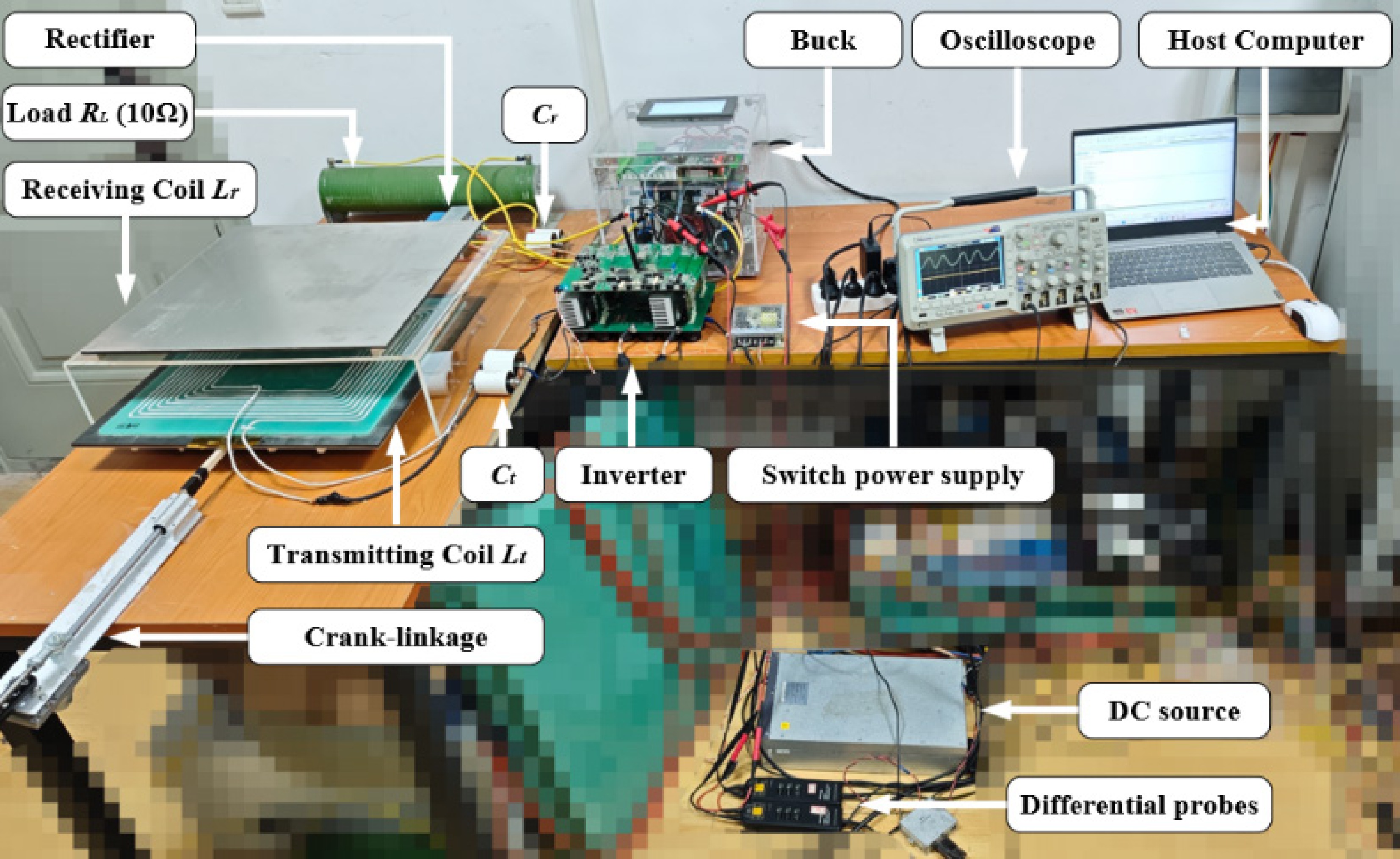
Figure 3. 

The prototype for experimental validation (with the coil lateral misalignment).

Notably, for the WPT system between offshore floating platforms, the mutual motion pattern of the coupling mechanism is specifically designed in this study, as illustrated in Fig. 4. To provide a more concrete illustration of these two modes of motion, the 3D model diagrams are constructed in Fig. 5. Lateral misalignment and angular variation of the coils are employed to simulate the mutual inductance fluctuation caused by wave-induced platform motions. The 50 cm × 50 cm square coils used are wound 10 turns by 0.1 × 800 Litz wire, with PC40 ferrite cores incorporated to reduce flux leakage. For lateral misalignment, a crank-linkage drives the transmitter coil to perform linear reciprocating motion with a maximum displacement of ± 10 cm, while the receiver coil remains stationary. For angular variation, with an acrylic slope as the back support, the transmitting coil is also driven by the crank-linkage, performs a reciprocating angular displacement with a maximum tilt angle of 11.3°.

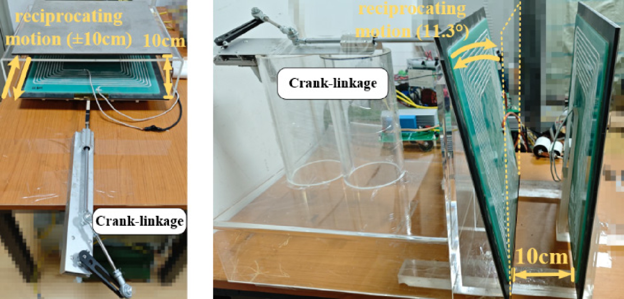
Figure 4. 

Implementation of coil lateral misalignment (left) and angular variation (right).

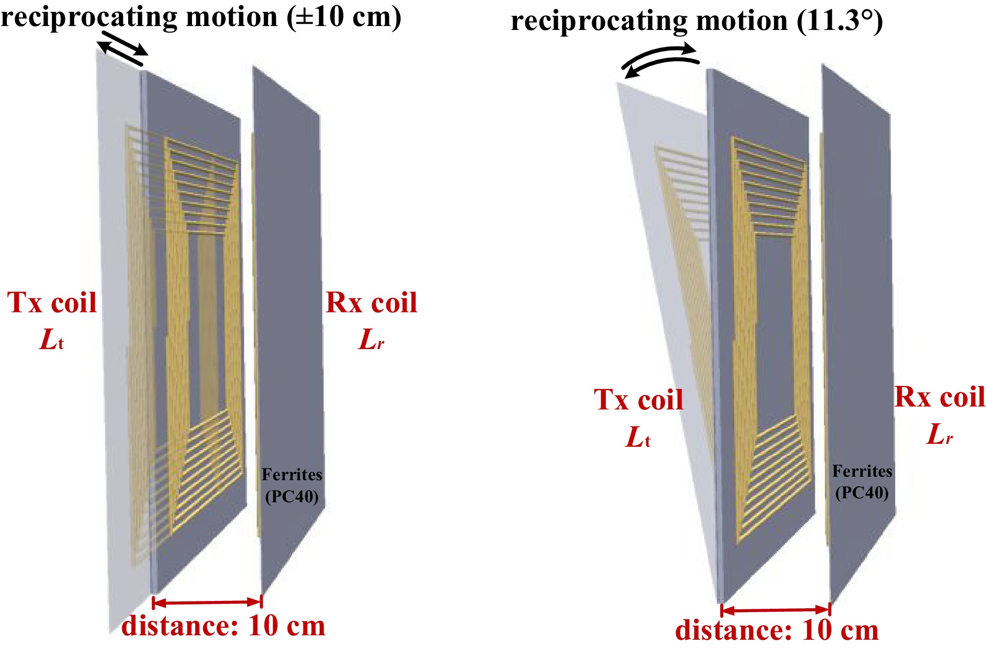
Figure 5. 

Schematic of the lateral misalignment (left) and angular variation (right).

Model identification and controller design

During model identification, the PRBS sequence with a 20 ms shift period, and ± 0.05 amplitude is injected into the duty cycle signal of the Buck under an open loop. Both the input voltage V_in, and output voltage V_out are sampled to form the dataset D_S = {V_out(k), D(k), V_in(k)}, with N = 6,500 and sampling interval 0.5 ms, as shown in Fig. 6. The LPV model parameters are then computed offline using the identification method described in above.

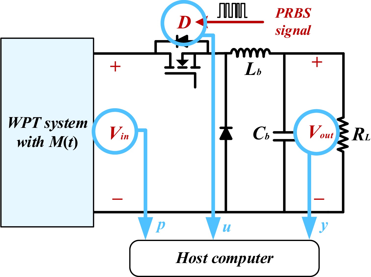
Figure 6. 

The PRBS injection and data sampling procedure.

The identified 2^nd-order LPV model of Buck is shown below, with a discretization period of 0.5 ms:

To evaluate model accuracy, the fitness index (FIT) calculated by the following equation is introduced, where $ {y}_{s} $is the simulated model output, $ {y}_{m} $ is the measured output, and $ {\overline{y}}_{s} $ is the mean of $ {y}_{s} $:

See Fig. 7 for the sampled dataset D_S = {V_out(k), D(k), V_in(k)} (1^st and 2^nd subplots) and the 90.72% FIT value of the model $ G({z}^{-1},k) $ 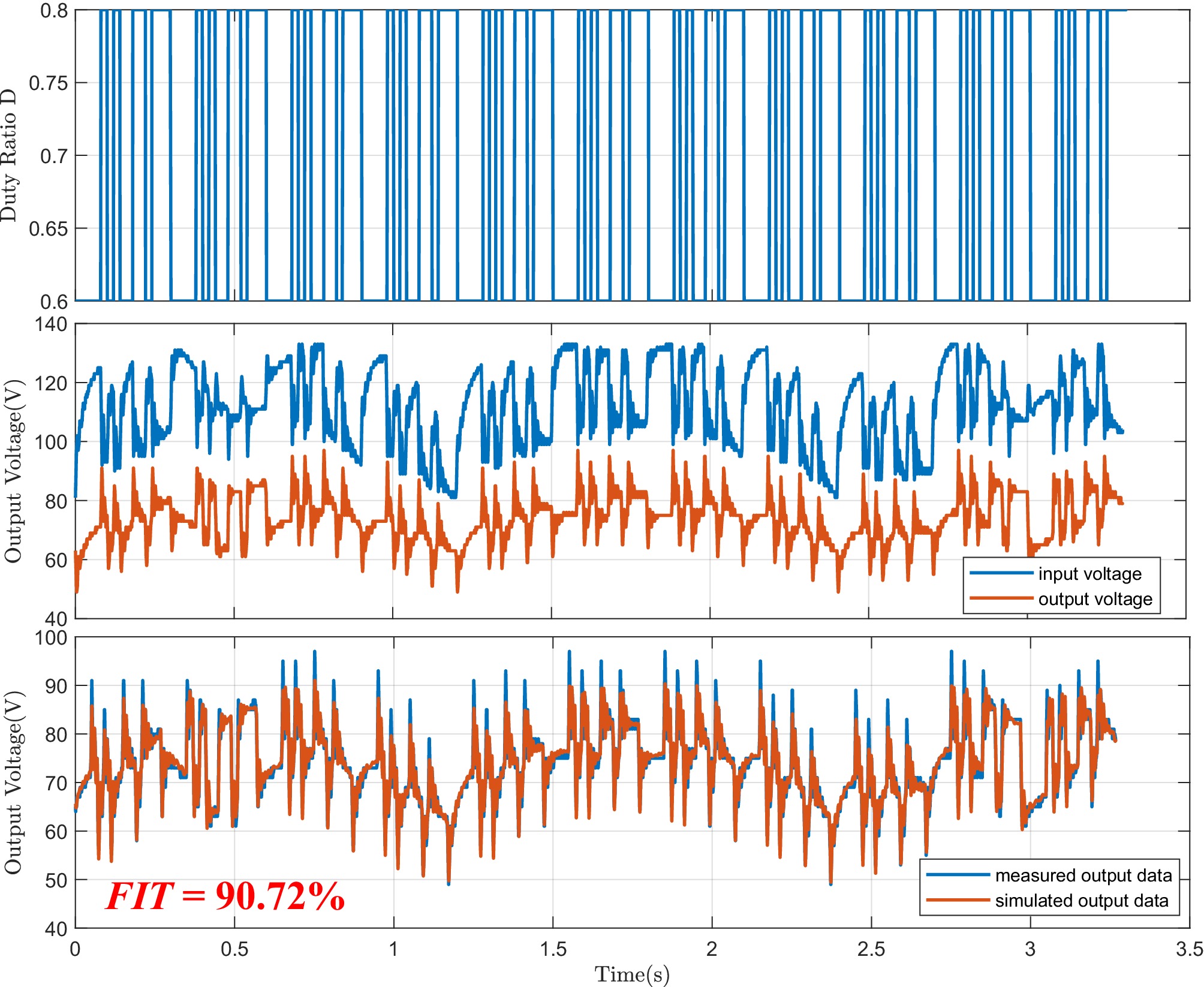of Eq. (24) (3^rd subplot), which indicates sufficient accuracy.

Figure 7. 

The sampled dataset D_S (1^st and 2^nd subplots), and the FIT value of the model G(z⁻¹, k) (3^rd subplot).

The MPC controller is designed based on model G(z⁻¹,k) identified as Eq. (24), with both the prediction horizon and control horizon set to 5 to reduce computational burden, and the weighting matrices Q and R are adjustable parameters.

Feasibility verification

Utilizing the aforementioned model and MPC controller, this study conducted experiments on constant-voltage output disturbance rejection control under both lateral misalignment and angular variation conditions of the WPT system coils.

lateral misalignment

Experiments are conducted under lateral coil misalignment as illustrated in Fig. 8, with the model in Eq. (24), and weighting matrices of MPC set to R = 100 and $ Q(k) = 7\times {10}^{-5}\cdot | {V}_{in}(k)-{V}_{in}(k- 1)| $. Fig. 8a, b presents the results of the WPT system maintaining a constant 100 V output under different motion frequencies (0.4 Hz, 0.7 Hz), with 1 kW transmission power to the load, and 85% overall machine efficiency. The overall machine efficiency incorporates all losses, which is defined and measured as follows: input power is measured at the DC power supply input, while output power is measured across the load resistance.

The V_out fluctuation, calculated by (V_in(max) − V_out(min))/ V_out(mean), remained within 3%, validating the effectiveness of the LPV modeling and MPC control. Furthermore, Fig. 8c, d shows the step response results, when V_out changed between 70 and 100 V, the setting time remained around 20 ms, indicating good dynamic performance. Finally, to verify control robustness, Fig. 8e, f demonstrates the result when the DC source voltage V_dc varied between 150 and 170 V. Evidently, variations in V_dc had nearly no effect on the constant output voltage, confirming excellent closed-loop robustness.

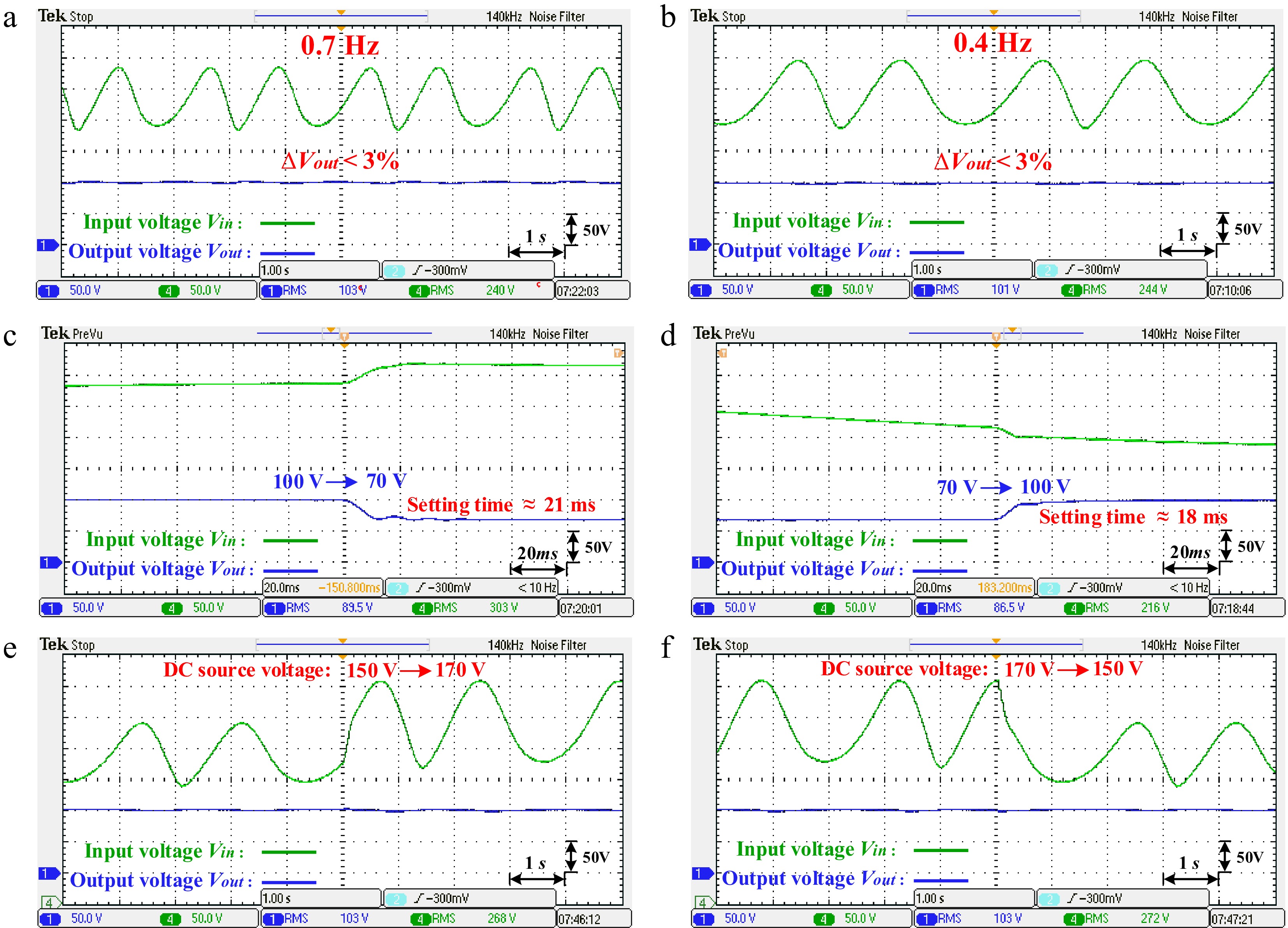
Figure 8. 

Experimental results under lateral coil misalignment. (a) Constant voltage output 100 V under motion frequency 0.7 Hz; (b) constant voltage output 100 V under motion frequency 0.4 Hz; (c) the step response results when V_out changed from 100 to 70 V; (d) the step response results when V_out changed from 70 to 100 V; (e) constant voltage output 100 V when DC source voltage V_dc changed from 150 to 170 V; (f) constant voltage output 100 V when DC source voltage V_dc changed from 170 to 150 V.

Angular variation

Similarly, experimental results under angular variation are shown in Fig. 9, with the same model from Eq. (24) and the MPC weighting matrices R = 100 and $ Q(k)=15\times10^{-5}\times\left|V_{in}(k)-V_{in}(k-1)\right| $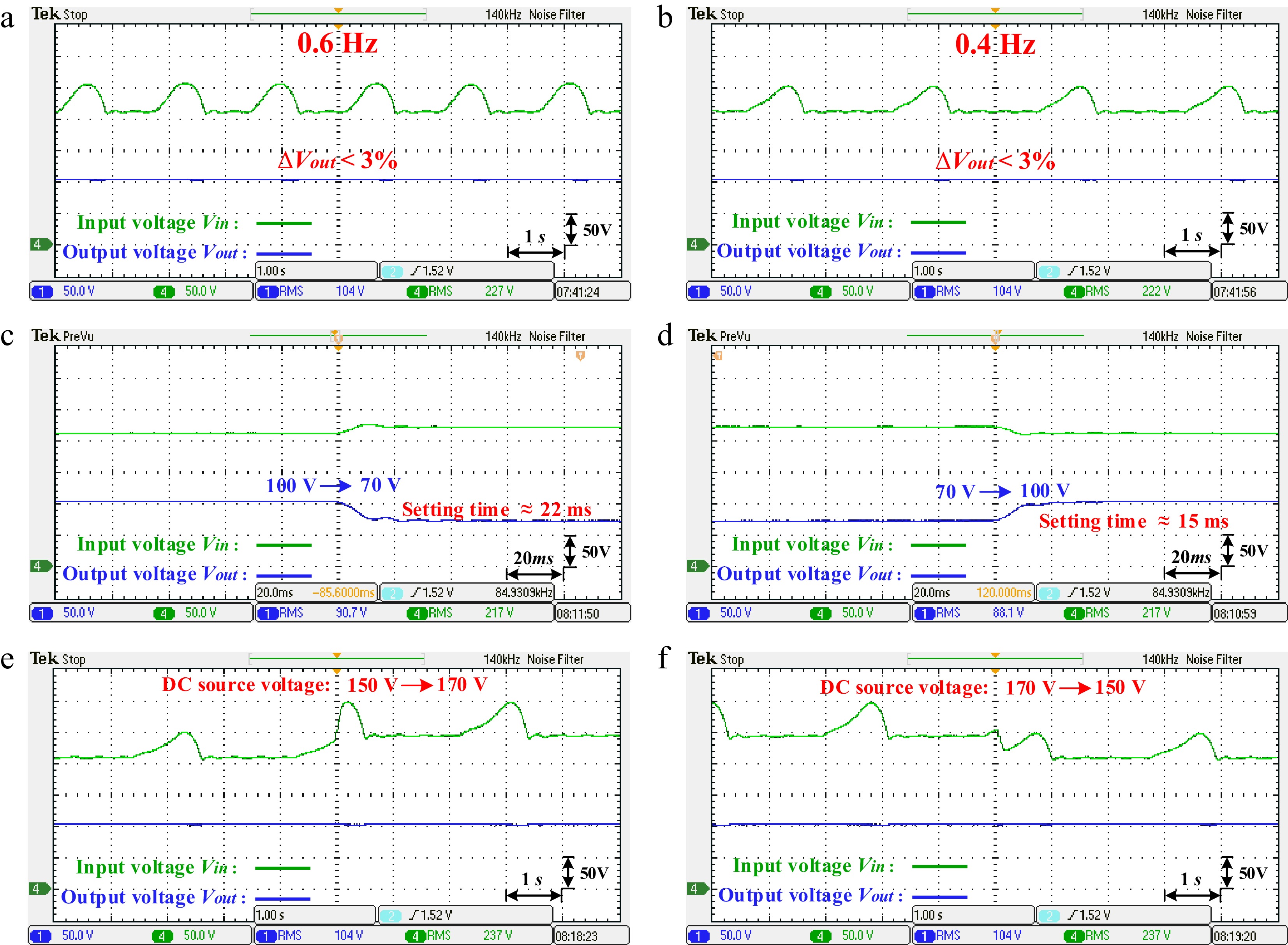. Fig. 9a, b presents the constant-voltage output performance test, Fig. 9c, d the dynamic performance test, and Fig. 9e, f the robustness test. All demonstrate satisfactory performance.

Figure 9. 

Experimental results under angular variation of coil. (a) Constant voltage output 100 V under motion frequency 0.6 Hz; (b) constant voltage output 100 V under motion frequency 0.4 Hz; (c) the step response results when V_out changed from 100 to 70 V; (d) the step response results when V_out changed from 70 to 100 V; (e) constant voltage output 100 V when DC source voltage V_dc changed from 150 to 170 V; (f) constant voltage output 100 V when DC source voltage V_dc changed from 170 to 150 V;

The proposed method features large-signal identification and modeling of Buck, but also presents potential limitations of open-loop identification. Closed-loop control is only implemented after the LPV model has been identified. On the other hand, since the LPV model of the Buck converter depends on the load resistance at the receiver side, any variation in the load resistance—such as that occurring in battery loads where the equivalent resistance changes with the state of charge—will alter the LPV model parameters. In such cases, the open-loop identification procedure must be repeated, which is both cumbersome and inconvenient.

Future work includes the introduction of a closed-loop parameter identification framework, which enables online updating of LPV model parameters during closed-loop operation when the receiver load changes. This approach eliminates the need for manual excitation injection and data sampling, thereby further enhancing the level of system automation.

In the WPT system with a receiver-side Buck converter, this paper introduces an integrated 'modeling + control' framework for large-signal LPV model identification of Buck converters and MPC controller design. Firstly, the LPV model accurately captures the nonlinear behavior of the Buck converter across a wide input voltage range, enabling the design of a linear controller for constant output voltage with effective disturbance rejection. Secondly, this approach eliminates the need to measure circuit component parameters, significantly enhancing practicality and operational convenience. Thirdly, the MPC strategy with time-varying weighting coefficients is adopted to implement disturbance rejection control for the LPV model, which avoids the design of complex robust controllers or tedious parameter tuning processes. Therefore, the proposed framework is highly suitable for disturbance-resistant wireless charging in unmanned offshore floating platforms.