Control barrier function-based obstacle avoidance and formation cooperative control for multi-UAV system with unknown disturbance

Owing to the advantages of fast flight speed and high robustness, the fixed-wing unmanned aerial vehicle (UAV) has gained widespread attention in various military and civilian fields^[1,2]. Meanwhile, compared with a single UAV, the multiple UAV system (MUAVS) has obvious superiority in large-scale search and confrontation tasks, such as forest fire patrol, collaborative target tracking, and cooperative surveillance^[3−5]. However, the safety control of MUAVS faces severe challenges and is worthy of long-term exploration.

Formation cooperative control is the primary problem to be solved for the safe flight of MUAVS, and a wide range of formation control approaches have been proposed in the existing literature. Guo et al.^[6] and Yildiz et al.^[7] developed the virtual structure-based formation control scheme for the UAV system to complete the tracking tasks with high quality. Peng et al.^[8] and Duan et al.^[9] proposed behavior-based methods to deal with the issues of dynamic task allocation and autonomous navigation, respectively. However, the virtual structure-based methods exhibit low fault tolerance and inflexibility. Meanwhile, the behavior-based methods struggle to ensure global performance. Consequently, this has driven the development of current consensus theory-based control technologies, with a considerable number of research outcomes having emerged. Shi et al.^[10] focused on the asynchronous consensus issue in discrete-time heterogeneous MUAVS, considering the effects of dynamic communication topologies. In terms of formation safety, Wu et al.^[11] put forward an improved consensus-based control algorithm to enhance the reliability of multi-UAV systems. By means of the multivariable adaptive control technique, Zhen et al.^[12] designed a consensus-based flight controller for the MUAVS in the presence of unknown uncertainty. By integrating directional communications with consensus-based coordination, Dong et al.^[13] constructed a distributed formation control framework for the multirotor UAV system. However, formation control is often coupled with autonomous obstacle avoidance, which poses new challenges to the task completion of UAV swarms.

Collision issues in the formation flight of MUAVS not only lead to mission failure but also cause property damage. Even worse, they may result in explosions and cause casualties. Therefore, various obstacle avoidance approaches have been proposed for the MUAVS in recent years, such as the rapidly exploring random tree method^[14], particle swarm optimization method^[15,16], and genetic algorithm^[17,18]. However, the aforementioned methods consider the UAV as mass points, ignoring the dynamic characteristics of the system itself. In contrast, the control barrier function (CBF) method has attracted widespread attention by explicitly formulating obstacle avoidance constraints and integrating them into the control law design in real time^[19]. Its essence lies in transforming obstacle avoidance from a path planning problem into a real-time control constraint problem, thus balancing system safety and task performance. Yin et al.^[20] addressed the pursuit–evasion game issue of multi-UAVs by virtue of the enhanced CBF technique. Peng et al.^[21] developed an innovative safe guidance method for the MUAVS in obstacle-rich environments by utilizing the high-order CBF. Ko & Chung^[22] constructed a feasibility-guaranteed filter for the robotic systems to ensure operational safety based on the backup CBF method. Ma et al.^[23] employed the discrete-time CBF for multi-rotor UAVs with limited sensory range to guarantee the robustness of the system during the learning and control stages. Moreover, the CBF approach is typically integrated with quadratic programming (QP), namely, the CBF-QP technique. Leveraging the optimization and solution capabilities of QP, a quantitative trade-off is achieved between 'satisfaction of safety constraints' and 'optimization of control performance', thereby significantly enhancing system performance. By means of the multiple Lyapunov functions method, Jang & Kim^[24] developed a CBF-QP-based control scheme for mobile robots to guarantee safe tracking in complex environments. Hung et al.^[25] designed a distributed tracking controller for MUAVS to achieve simultaneous occlusion and collision avoidance in light of the CBF-QP technique. Combining the CBF and QP methods, Yan et al.^[26] presented an innovative iterative learning algorithm for a multi-agent system performing repetitive tasks to maintain the output safety of agents throughout every iteration. However, practical flight environments inevitably expose the MUAVS to unknown disturbances, which may degrade obstacle avoidance performance and even induce system instability.

To overcome this problem, many disturbance rejection schemes have been proposed over the past few decades, including the extended state observer (ESO)^[27] and the disturbance observer^[28]. However, the two aforementioned methods employ the estimated values for compensation after the observation error converges, while their control performance remains uncertain before the error converges. In contrast, the interval disturbance observer (IDO) can provide the upper and lower bounds of disturbance and encompass all possible values at any time, thereby guaranteeing its widespread application. Yong et al.^[29] combined the IDO with the sliding mode control method for nonlinear systems to handle the problem of disturbance rejection. Luo et al.^[30] proposed a distributed IDO for discrete-time multi-agent systems with unknown uncertainties to achieve coordination control. Wang et al.^[31] developed a robust coordination control scheme for multi-agent systems based on the distributed IDO. In order to achieve safe formation flight, Ma et al.^[32] presented an asymptotic consensus control strategy for the linear multi-agent systems based on the IDO method. Zhu et al.^[33] introduced a set of IDOs for a quadrotor UAV with a cable-suspended load to enhance disturbance robustness and improve fault sensitivity. Yong et al.^[34] explored the problem of tracking control for uncertain nonlinear systems under intense external disturbances to guarantee operational reliability. However, the coordinated control problem involving obstacle avoidance, formation maintenance, and anti-disturbance remains to be explored in depth.

Motivated by the above discussion, a CBF-QP-based cooperative formation control scheme with obstacle avoidance capability is designed for MUAVS under unknown disturbances. The main contributions are outlined below:

(1) Compared with the existing ESO and conventional disturbance observer methods, the proposed IDO provides real-time upper and lower bound estimations of the unknown disturbance. In this way, unknown disturbances can be enveloped at any time rather than only after the observation errors converge, which improves the disturbance rejection capability and safety performance of the MUAVS.

(2) Compared with the traditional obstacle avoidance methods that treat UAVs as mass points, the proposed CBF-QP-based method incorporates obstacle avoidance constraints into the real-time controller design, which achieves an effective trade-off between safe tracking performance and dynamic optimization.

(3) A robust formation obstacle avoidance control framework is developed by integrating IDO, consensus theory, and CBF-QP. The proposed control mechanism can not only meet the performance requirements for formation obstacle avoidance but also enhance the disturbance rejection capability of the entire MUAVS.

This paper is structured in the following manner. The section "Problem formulation and preparation" establishes the nonlinear dynamic model for fixed-wing MUAVS and introduces the necessary theoretical preliminaries. The detailed design procedure of the IDO and CBF-QP formation obstacle avoidance controller is elaborated in the section "Controller design and stability analysis". In the "Simulation results" section, the numerical simulation outcomes are presented to verify the effectiveness of the proposed control scheme. The section "Conclusions" summarizes the core findings and outlines future research prospects.

Notations: In this work, $ {R_n} $ and $ {R_{n \times m}} $ denote the $ {n} $-dimensional Euclidean space and the set of $ {n \times m} $ matrices, and $ {R_ + } = \{ x \in R:x \ge 0\} $. $ {{I_n}} $ denotes the $ {n \times n} $ identity matrix. $ {diag\{ {c_1}, \cdots ,{c_i}\}} $ represents the diagonal matrix with diagonal entries $ {{c_i}} $. $ {{\lambda _{\max }}( \cdot )} $ stands for the maximum eigenvalues. The symbol $ {\otimes} $ denotes the Kronecker product, and $ {1_n} \in {R^{n \times 1}} $ is the unit column vector.

Consider a MUAVS consisting of $ n $ UAVs. The information exchange among them is described by the directed graph

where $ v_r = \{v_{r1},v_{r2},\dots,v_{rn}\} $ is the node set, with each node corresponding to an individual UAV, and $ \varepsilon_r = \{(v_{ri},v_{rj}): v_{ri},v_{rj}\in v_r\} $ is the edge set, indicating the direction of information transmission between UAVs. The topological structure is further characterized by the adjacency matrix $ A_r = (a_{ij})\in {R}^{n\times n} $. Specifically, $ a_{ij} = 1 $ if node $ j $ receives information from node $ i $, and $ a_{ij} = 0 $ otherwise. Self-loops are excluded, i.e., $ a_{ii} = 0 $. The degree matrix is given by $ D_r = diag\{d_{r1},\dots,d_{rn}\} $, with $ d_{ri} = \sum_{j = 1}^n a_{ij} $. Consequently, the Laplacian matrix of $ G_r $ is defined as $ L_r = D_r-A_r $.

For the leader-follower scenario, the augmented graph $ \bar G_r = (\bar v_r,\bar\varepsilon_r) $ and the pinning matrix $ S = diag\{s_1,\dots,s_n\} $ are introduced, where $ s_i = 1 $ if the $ i $-th follower can access the leader's state, and $ s_i = 0 $ otherwise.

CBF and QP

Definition 1^[24]: A continuous function $ {\wp :[0,\alpha ) \to [0,\infty )} $ qualifies as a class $ {K} $ function for $ {\alpha \gt 0} $, if it is monotonically increasing and $ {\wp (0) = 0} $.

Definition 2^[22,24]: Consider a control system as follows:

where $ {\eta \in {R^n}} $ denotes the system state, $ {f:{R^n} \to {R^n}} $ and $ {g:{R^n} \to {R^{n \times q}}} $ are known nonlinear locally Lipschitz continuous functions, and $ {u \in {R^q}} $ is the control input.

For a solution $ {\eta (t)} $ of system (2), if the initial state satisfies $ {\eta ({t_0}) \in C \subset {R^n}} $, it guarantees that $ {\eta (t) \in C} $ holds for all $ {t \ge {t_0}} $. Then, the set $ {C} $ is called the forward invariant set with respect to system (2).

Definition 3^[22,23]: For a continuously differentiable function $ {{ -\!\!\!\!\lambda} :{R^n} \to R} $, if there exists a class $ {K} $ function $ {\wp } $ satisfying

where $ {U} $ denotes the admissible set of control inputs, $ {{L_f}} $ and $ {{L_g}} $ represent the Lie derivative operators with respect to the vector fields $ {f(x)} $ and $ {g(x)} $, respectively. Then $ {{ -\!\!\!\!\lambda} } $ is called a CBF for system (2).

Based on Definition 2, the optimal controller for system (2) can be obtained by solving the following QP problem:

Problem description

For ease of presentation, the schematic illustration of the fixed-wing UAV structure is provided in Fig. 1, where $ {\chi} $, $ {\gamma} $, and $ {\mu} $ are the course yaw angle, course pitch angle, and course roll angle, respectively. $ {({O_b},{X_b},{Y_b},{Z_b})} $ denotes t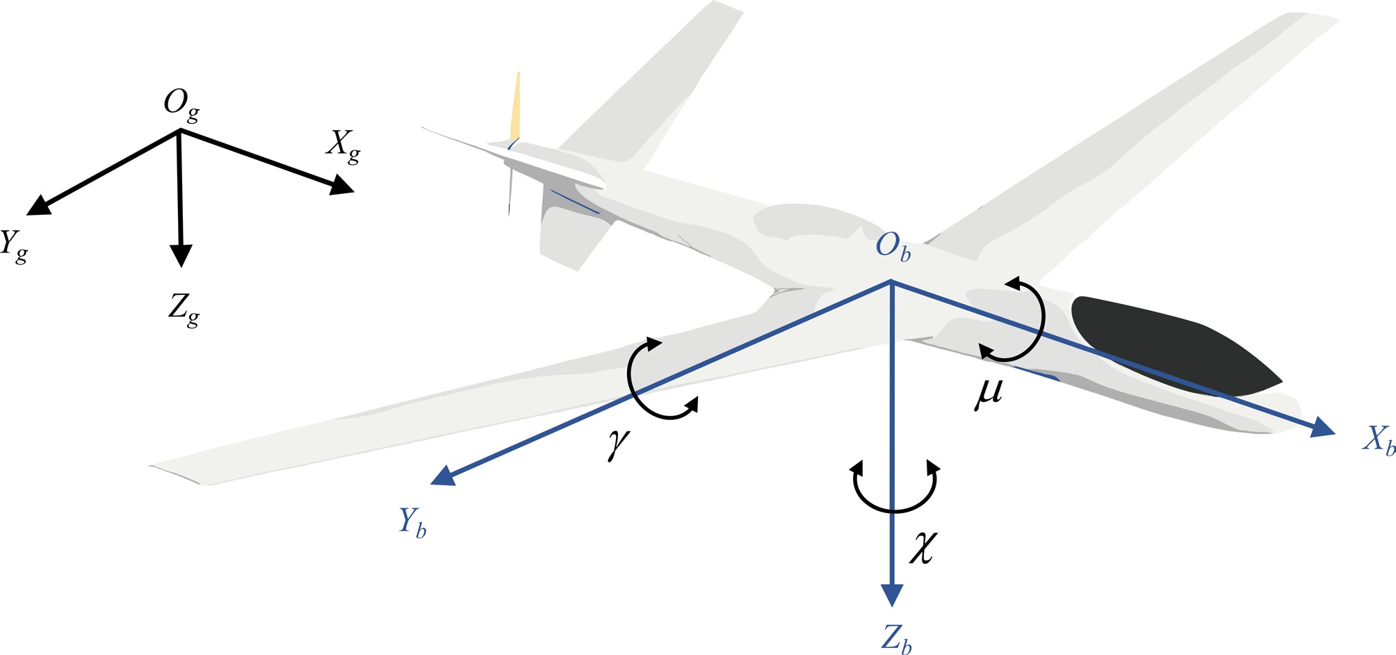he body frame and $ {({O_g},{X_g},{Y_g},{Z_g})} $ refers to the inertial frame. Based on Newton's second law, a simplified dynamic model for any UAV within the formation in three-dimensional space can be described as^[35]

Figure 1. 

The structure of fixed-wing UAV.

where $ m $ is the UAV mass and $ g $ the gravitational acceleration. For the $ i $th fixed-wing UAV, its inertial position $ (x_i,y_i,z_i) $, speed $ V_i $, heading angle $ \chi_i $, and flight-path angle $ \gamma_i $ constitute the state variables, while the lift $ L_i $, thrust $ T_i $, and course roll angle $ \mu_i $ serve as the control inputs.

For simplifying the control design, we define an equivalent input vector $ u_i = [u_{xi}, u_{yi}, u_{zi}]^T $ by setting $ u_{xi} = T_i/(mg) $, $ u_{yi} = L_i\sin\mu_i/(mg) $, and $ u_{zi} = L_i\cos\mu_i/(mg) $. Evidently, the actual inputs $ L_i, T_i, \mu_i $ are recoverable from the equivalent one $ u_i $. When external disturbances are also accounted for, the dynamic model (5) of the $ i $th fixed-wing UAV is rewritten as

where $ {\ell _i} = {[{x_i},{y_i},{z_i}]^T} $ is the position vector, $ {{d_i} = {[{d_{ix}},{d_{iy}}, {d_{iz}}]^T}} $ represents the unknown disturbance, $ {\dot \varsigma _i} = {\ddot \ell _i} = {[{\ddot x_i},{\ddot y_i},{\ddot z_i}]^T} $, $ {F_i} = {[0,0, - g]^T} $, and

Here, the unknown disturbance $ {d_i} $ is generated by the following exogenous system

where $ {{\delta _i} \in {R^{3\times 1}}} $ is the state vector, $ {{A_i}\in {R^{3\times 3}}} $, $ {{B_i} \in R_ + ^{3\times 1}} $ and $ {{C_i}\in R_ + ^{3\times 3}} $ are the known constant matrices, $ {{\varpi _i}} $ denotes the unknown bounded input vectors satisfying $ {{\varpi _i} \le \varpi _i^ * } $ with a known positive constant vector $ {\varpi _i^ * } $, $ {i = 1,2, \cdots ,N} $.

This study focuses on the design of a formation control scheme with obstacle avoidance capability, which allows MUAVS to effectively reject disturbances while ensuring safe distances to obstacles. In light of this, several necessary assumptions and related lemmas are introduced.

Assumption 1^[29,36]: For any $ {x \in {R^n}} $, there exists a smooth nonlinear function $ {H(x):{R^n}\to} {{R^m}} $ such that $ {\dfrac{{\partial H(x)}}{{\partial x}}} $ exists.

Assumption 2^[31]: Consider a directed graph $ G_r $ and its Laplacian $ L_r \in {R}^{n \times n} $. When $ G_r $ has a directed spanning tree, the following hold: zero is a simple eigenvalue of $ L_r $, the right eigenvector for this zero eigenvalue has only nonnegative entries, and every other eigenvalue has strictly positive real part.

Assumption 3^[34,36]: The external disturbance $ {d_i} $ is unknown and bounded, satisfying $ {\left\| {{d_i}} \right\| \le {d_{im}}} $, where $ {d_{im}} \in {R_+ } $.

Assumption 4: In the cruise phase of the fixed-wing UAV, the sideslip angle and angle of attack are assumed to be zero. Meanwhile, the lateral force and drag can be safely ignored in the presence of the dominant lift force.

Lemma 1^[31,34]: Consider the system $ {\dot s(t) = {q_s}s(t) + {\omega _s}(t)} $ with $ {{q_s} \in {R^{n \times n}}} $ being the state vector and $ {{\omega _s}(t) \in R_ + ^n} $ being a time-varying vector. If $ {q_s} $ is a Metzler matrix for all $ {t \ge 0} $, then the condition $ {{q_s}(t) \in R_ + ^n} $ also holds for all $ {t \ge 0} $.

Lemma 2^[29]: Design a matrix $ {Q_s} \in {R^{n\times n}} $ such that the matrix $ {\left( {{A_s} - {Q_s}{C_s}} \right)} $ has same eigenvalue with a Metzler and Hurwitz matrix $ {H_s} \in {R^{n\times n}} $, where $ {{A_s},{C_s} \in {R^{n \times n}}} $. If there exist two vectors $ {q_{1} \in {R^{1\times n}}} $ and $ {q_{2}\in {R^{1\times n}}} $ such that the pairs $ {\left( {{A_s} - {Q_s}{C_s},{q_{1}}} \right)} $ and $ {({H_s},{q_{2}})} $ are observable, then $ {W_s^{ - 1} = O_{2s}^{ - 1}{O_{1s}}} $ and $ {{\Gamma _s} = W_s^{ - 1}{Q_s}} $, where

Remark 1: For any smooth nonlinear functions, their partial derivatives always exist, so Assumption 1 is reasonable. Assumption 2 is a common assumption in the research of UAV swarm formation control and can be easily satisfied under practical UAV communication topologies. In practical systems, external disturbances always have bounded energy. Otherwise, no controller can suppress disturbances with infinite energy, which demonstrates the rationality of Assumption 3. During the cruise flight of fixed-wing UAVs, there is no sideslip of the airframe and the pitch angle is nearly horizontal. Meanwhile, the lateral force and drag force are far smaller than the lift force. Therefore, Assumption 4 is also reasonable. Assumptions 1–4 above are widely adopted in formation control and can be found in many existing literature^{[21,29,34,36]}.

In this section, the proposed control scheme for MUAVS under unknown disturbances is formulated, which contains three core components: the IDO, the consensus-based formation control, and the CBF-QP-based obstacle avoidance strategy. For clearer illustration, the control flow block diagram of the proposed method is provided in Fig. 2.

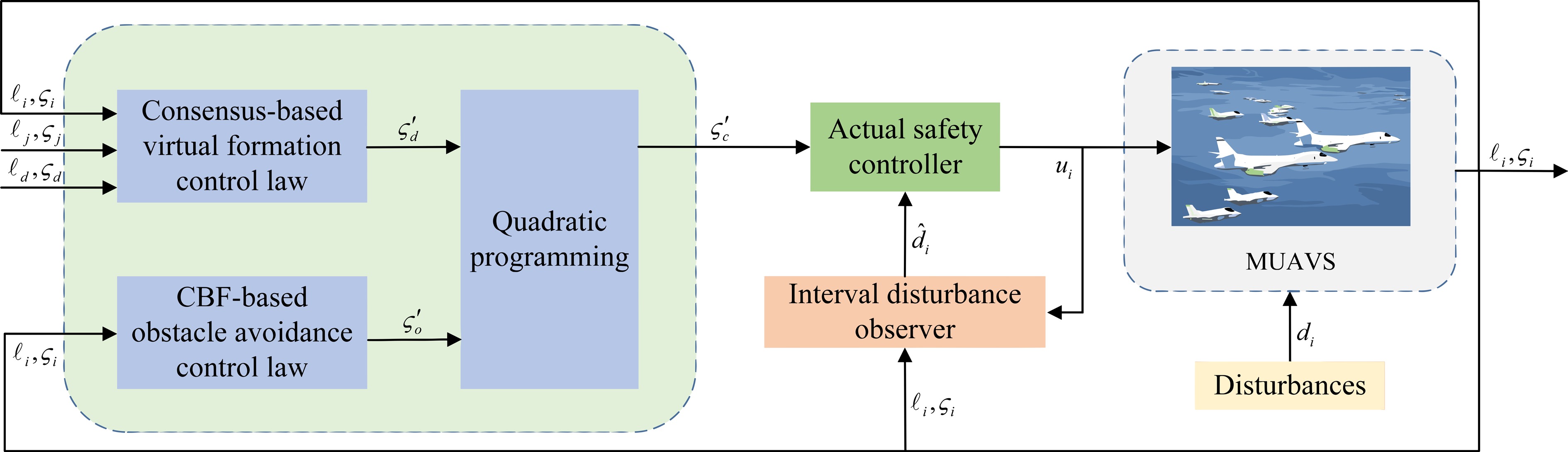
Figure 2. 

Control flow block diagram of the proposed method.

The design of IDO

For the established affine nonlinear model (6) of MUAVS, the IDO designed in this subsection can effectively compensate for the impact of unknown disturbance. To facilitate the design of the IDO, an auxiliary variable $ {\psi _i} \in {R^{3\times 1}} $ is introduced as^[29]

where $ {{W_i}\in {R^{3\times 3}}} $ is a designed constant matrix, and $ {\vartheta ({{\varsigma }_i})} $ is a designed nonlinear function related to $ \varsigma_i $, $ {i = 1,2, \cdots ,N} $.

Considering (6), (8) and (10), the derivative of $ {{\psi _i}} $ satisfies

where

Here, according to Assumption 1, the nonlinear function vector $ {\vartheta ({{\varsigma }_i})} $ can be designed as $ {\vartheta ({{\varsigma }_i}) = {Q_i}\varsigma_i} $, which indicates that

where $ {Q_i} \in {R^{3\times 3}} $ is a designed constant matrix.

Then the auxiliary variable can be expressed as

The IDO can be designed by estimating the upper boundary $ {{\bar \psi _i}} $ and lower boundary $ {\underline{\psi } _i} $ of the auxiliary variable, which is constructed as follows:

Define the estimation errors of the upper boundary as $ {{\bar z_{\psi i}} = {\bar \psi _i} - {\psi _i}} $, and the estimation errors of the lower boundary as $ {{\underline z_{\psi i}} = {{\psi _i} - \underline{\psi } _i}} $. Differentiating $ {{\bar z_{\psi i}}} $ and $ {{\underline z_{\psi i}}} $ and considering (15) and (16), we have

Remark 2: In this step, for a given vector $ {L = {\left[ {{l_1}, \cdots ,{l_n}} \right]^T}} $, define $ {\left| L \right| = {\left[ {\left| {{l_1}} \right|, \cdots ,\left| {{l_n}} \right|} \right]^T}} $. Taking (17) for example and assuming that $ {W_i^{ - 1}{B_i} = {\left[ {{l_{w1}}, \cdots,{l_{wn}}} \right]^T}} $, we have $ {\left| {W_i^{ - 1}{B_i}} \right| = } { {\left[ {\left| {{l_{w1}}} \right|,\cdots ,\left| {{l_{wn}}} \right|} \right]^T}} $.

From the aforementioned analysis, the following theorem is derived:

Theorem 1: Consider the nonlinear system (6) under bounded disturbance given by (8). From the designed IDO (15) and (16), the intervals of the disturbance are given by

where $ {(W_i^{ - 1})^ + } = \max ({W_i^{ - 1}},O) $ and $ {(W_i^{ - 1})^ - } = {(W_i^{ - 1})^ + } - (W_i^{ - 1}) $ with $ {O} $ being the zero matrix.

Furthermore, if the matrix $ {W_i^{-1}\left( A_i - Q_i C_i \right) W_i} $ is Hurwitz and Metzler, and the boundary estimation errors $ {\bar z_{di}} = {\bar d_i} - {d_i} $ and $ {\underline z_{di}} = {d_i}-{\underline d_i} $ are always nonnegative and bounded, and the initial conditions that $ {\bar z_{\psi i}}(0) $ and $ {\underline z_{\psi i}}(0) $ are nonnegative.

Proof: The dynamics of boundary estimation errors $ \dot{\bar{z}}_{\psi i} $ and $ \dot{\underline{z}}_{\psi i} $ can be written as

where $ {{H_i} = W_i^{ - 1}\left( {{A_i} - {Q_i}{C_i}} \right){W_i}} $, $ {\bar \Psi _i} = \left| {W_i^{ - 1}{B_i}} \right|\varpi _i^ * - W_i^{ - 1}{B_i}{\varpi _i} $ and $ {\underline \Psi _i} = \left| {W_i^{ - 1}{B_i}} \right|\varpi _i^ * + W_i^{ - 1}{B_i}{\varpi _i} $.

According to Lemma 1, an appropriate matrix is chosen such that $ {{H_i} = W_i^{ - 1}\left( {{A_i}- {Q_i}{C_i}} \right){W_i}} $ is Hurwitz. Namely, the following equation holds:

where $ {{K_i}} $ and $ E_i $ are the positive definite matrix.

Select the Lyapunov function $ {V_1} $ as

By invoking (21) and (22), taking the time derivative of $ {V_1} $ yields

where $ \left\| {\bar \Psi _i^T{E_i}} \right\| \le {\bar \lambda _{di}} $ and $ \left\| {\underline \Psi _i^T{E_i}} \right\| \le {\underline \lambda _{di}} $.

Considering (21) and (22), the disturbance estimation errors can be further written in the following form:

where $ {{\Phi _i} = \Phi _i^ + - \Phi _i^ - } $, since $ {{C_i} \ge 0} $, $ {{\Phi _i^ +} \ge 0} $, $ {{\Phi _i^ -} \ge 0} $, $ {{\bar z_{\psi i}}} $ and $ {{\underline z_{\psi i}}} $ are non-negative and bounded, the disturbance estimation errors $ {{\bar z_{d i}}} $ and $ {{\underline z_{d i}}} $ are non-negative and bounded, that is, the true disturbance $ {d_i} $ satisfies $ {\underline d_{i}}\le{d_i}\le{\bar d_{i}} $.

In this step, the key lies in selecting adequate matrices such that $ {H_i} $ is Metzler and Hurwitz stable. According to Lemma 2, $ {H_i} $ can be computed by solving a Sylvester equation: $ {W_i^{-1} A_i - H_i W_i^{-1} = {\Gamma _i}C_i} $, $ {{\Gamma _i} = W_i^{ - 1}Q_i} $, where $ {H_i} $ and $ {A_i} $ share the same eigenvalue^[37].

Remark 3: Since the estimation errors $ {\bar z_{di}} $ and $ {\underline z_{di}} $ are always nonnegative and bounded in Theorem 1, we can obtain that $ {z_{di}^ * = {{\bar z}_{di}} + {{\underline z}_{di}} = {{\bar d}_i} - {{\underline d}_i}} $ is also bounded. Applying the inequality condition, it follows that $ {- \frac{1}{2}({{\bar d}_i} - {{\underline d}_i}}) \le {d_i} - {{\hat d}_i} \le \frac{1}{2}({{\bar d}_i} - {{\underline d}_i}) $, which means that $ {z_{di}} = {d_i} - {{\hat d}_i} $ is bounded, $ {i = 1,2, \cdots ,N} $.

Consensus-based virtual formation control design

The tracking position error $ {{z_{\ell i}}} $ and velocity error $ {{z_{\varsigma i}}} $ of the $ {i} $th follower UAV are defined as^[38]

where $ {{z_{\ell i}} = {[{z_{\ell ix}},{z_{\ell iy}},{z_{\ell iz}}]^T}} $ and $ {{z_{\varsigma i}} = {[{z_{\varsigma ix}},{z_{\varsigma iy}},{z_{\varsigma iz}}]^T}} $ represent the position error and velocity error of the $ i $th UAV in the three-axis directions, respectively. $ a_{ij} $ and $ s_i $ are the adjacency weight among followers and the pinning weight from the leader. $ \kappa_{ij} = \kappa_{id}-\kappa_{jd} $ is the desired offset between the $ i $UAV and $ j $UAV with $ \kappa_{id} = \ell_i-\ell_d $ and $ \kappa_{jd} = \ell_j-\ell_d $, $ \ell_i $ and $ \varsigma_i $ are the position and velocity of the $ i $th follower UAV, $ \ell_d $ and $ \varsigma_d $ are those of the leader UAV.

Applying algebraic operations to (28) and (29) yields

where $ {{L_\ell } = ({L_r} + S) \otimes {I_3}} $, $ {{L_r} \in {R^{n \times n}}} $ denotes the follower sub-graph Laplace matrix, $ {S = diag} {{\{s_1}, \cdots {s_i}\} } $ is the leader-follower communication weight matrix with $ {{s_i} \gt 0} $. Since $ {L_r} $ is positive semi-definite and $ {S} $ is a positive diagonal matrix with at least one positive entry, $ {({L_r} + S)} $ is positive definite and thus invertible, which implies the invertibility of $ {L_\ell } $. $ {{z_\ell } = {[{z_{\ell 1}}, \ldots ,{z_{\ell i}}]^T}} $, $ {{z_\varsigma } = {[{z_{\varsigma 1}}, \ldots ,{z_{\varsigma i}}]^T}} $, $ {\ell = {[{\ell _1}, \cdots ,{\ell _i}]^T}} $, $ {\varsigma = {[{\varsigma _1}, \cdots ,{\varsigma _i}]^T}} $, $ {{\kappa} = {[{\kappa _{1}}, \ldots ,{\kappa _{i}}]^T}} $, $ {{\ell '_d} = {1_n} \otimes {\ell _d}} $, $ {{\varsigma '_d} = } { {1_n} \otimes {\varsigma _d}} $, $ {i = 1,2, \cdots ,N} $.

Taking the derivative of $ {z_\ell } $ produces

Design virtual formation control input as

where $ {{\lambda _\ell } = diag\{ {\lambda _{\ell 1}}, \cdots ,{\lambda _{\ell i}}\} } $ is the designed positive definite matrix, and $ {{\lambda _{\ell i}} = diag\{ {\lambda _{\ell ix}},} {{\lambda _{\ell iy}},{\lambda _{\ell iz}}\} } $, $ {i = 1,2, \cdots ,N} $.

By substituting (33) into (32), we obtain

Subsequently, the Lyapunov function candidate is selected as

Invoking (34), we have

CBF-QP-based obstacle avoidance and formation cooperative control design

The function of CBF is to guarantee a safety margin between the position of the UAVs and obstacles. To avoid collision avoidance between the UAVs and obstacles, the safety set $ {C_{bi}} $ for the $ i $th UAV is defined as

where $ {{h_i}(\ell )} $ is regarded as a CBF for the $ i $th UAV with the form of^[20]

where $ {{\ell _{oi}} = {[{\ell _{oix}},{\ell _{oiy}},{\ell _{oiz}}]^T}} $ represents the three-axis positions of multiple obstacles, and $ {{d_{safe}}} $ represents the safe distance of the avoidance area.

Design $ {h(\ell ) = {\left[ {{h_1}(\ell ), \cdots ,{h_i}(\ell )} \right]^T}} $ as the CBF of the entire MUAVS. Clearly, it can be further expressed as

Based on (6), the time derivative of (39) can be obtained as

where $ {{L^o} = diag\left\{ {{{({\ell _1} - {\ell _{o1}})}^T}, \cdots ,{{({\ell _i} - {\ell _{oi}})}^T}} \right\}} $.

The core function of QP is to efficiently solve for the optimal control input that meets the obstacle avoidance requirements under the safety constraints provided by the CBF, while balancing the UAV's mission objectives and dynamic constraints. Combining CBF and QP, the virtual safety control law $ {\varsigma_c} $ is defined as

where $ {\varsigma_c = {[{\varsigma _{c1}}, \cdots ,{\varsigma _{ci}}]^T}} $.

Remark 4: Here, each $ \dot h_i(\ell ) \ge 0 $ serves as the constraint condition for $ \mathop {\min }\limits_{{\rm{ }}{{\varsigma_i}}} {\left\| {{{\varsigma_i}} - {{\varsigma'_{di}}}} \right\|^2} $, where $ \varsigma'_{di} $ is the $ i $^th element of $ \varsigma'_{d} $. Then, the virtual safety control law $ \varsigma_{ci} $ for each UAV can be derived. Therefore, for the whole MUAVS consisting of $ i $ UAVs, the resulting virtual safety control law is $ \varsigma_c = [\varsigma_{c1},\cdots, \varsigma_{ci}]^T $.

Define the error between the virtual safety control law $ {\varsigma_c} $ and the virtual formation control law $ {\varsigma'_d} $ as $ {{z_c} = {\varsigma _c} - {\varsigma '_d}} $. In this work, the error $ {z_c} $ and its first-order derivative are assumed to be bounded, namely, there exist positive constants making $ {\left\| {{z_c}} \right\| \le {\delta _c}} $ and $ {\left\| {{{\dot z}_c}} \right\| \le {\delta _\Theta }} $ hold^[19].

Remark 5: The boundedness assumptions for the error between the virtual safety control law $ {\varsigma_c} $ and the virtual formation control law $ {\varsigma'_d} $, as well as its time derivative, are reasonable and well-founded. The CBF-QP constraint confines the system state to the predefined safe set, ensuring the boundedness of $ {\varsigma_c} $. Combined with the boundedness of $ {\varsigma'_d} $ and its derivatives, the error and its derivative are consequently bounded. Such assumptions are common and acceptable in the stability analysis of constrained formation control systems.

Differentiating $ {z_\varsigma } $ yields

where $ {F = {[{F_1},\cdots,{F_i}]^T}} $, $ {G = diag\left\{ {{G_1},\cdots,{G_i}} \right\}} $, $ {u = {[{u_1}, \cdots , {u_i}]^T}} $, $ {d = {[{d_1}, \cdots,{d_i}]^T}} $, $ {i = } {1,2, \cdots ,N} $.

Invoking (41) and (42), the resulting obstacle avoidance and formation cooperative controller is designed below:

where $ {{\lambda _\varsigma } = diag\{ {\lambda _{\varsigma 1}}, \cdots ,{\lambda _{\varsigma i}}\} }>0 $, and $ {{\lambda _{\varsigma i}} = diag\{ {\lambda _{\varsigma ix}},}{{\lambda _{\varsigma iy}},{\lambda _{\varsigma iz}}\} } $, $ {\hat d = {[{\hat d_1}, \ldots ,{\hat d_i}]^T}} $, $ {\hat d_i} = \frac{1}{2}({\bar d_{i}}+{\underline d_{i}}) $ is the disturbance estimation value, $ {i = 1,2, \cdots ,N} $.

By substituting (43) into (42), we obtain

Choose the Lyapunov candidate function $ {V_3} $ as

Considering (34) and (44), it gives

where $ {z_d} = {[{z_{d1}}, \cdots ,{z_{di}}]^T} $ is the bounded estimation errors, $ {\left\| {{\dot z}_c} \right\| \le {\delta _\Theta}} $, $ {\left\| {z_d} \right\| \le {\delta _{d}}} $, where $ {{\delta _\Theta}} $, $ {{\delta _{d}}} $ are positive constants, $ {{{\bar \lambda }_\varsigma } = {\lambda _\varsigma } - {I}} $, $ {I \in {R^{3n \times 3n}}} $, $ {i = 1,2, \cdots ,N} $.

According to the definition of the controller in dynamic system (6), the actual control inputs are obtained as follows:

Stability analysis

Overall, the above analysis can be stated as the following theorem:

Theorem 2: For the nonlinear model (6) of MUAVS with unknown disturbance, the IDO is designed as (15) and (16). Under the proposed safe formation and obstacle avoidance flight controller (43), all error signals of the whole MUAVS are ultimately uniformly bounded, and the follower UAV can effectively track the leader UAV.

Proof: Let $ V_4 = V_1+V_3 $ be a Lyapunov candidate. Then, differentiating it and applying (25) and (46) yields

where $ {{\varepsilon _0} = \min \left\{ {\dfrac{{{K_i} - {I_i}}}{{{\lambda _{\max }}{E_i}}},2{\lambda _\ell },2{{\bar \lambda }\varsigma }} \right\}} $, $ {{\varepsilon _1} = \bar \lambda _{di}^2 + \underline\lambda_{di}^2 + \dfrac{1}{2}{\delta^2_\Theta} }+ \dfrac{1}{2}{{\delta^2_d}} $.

Integration of (48) produces

According to (49), $ {V_4} $ gradually converges as time goes on, which indicates that all error signals in the closed-loop system are ultimately uniformly bounded. This concludes the proof.

Remark 6: The stability of the system is further enhanced by the synergistic operation of the IDO and CBF-QP. The disturbance compensation provided by the IDO enables the CBF-QP-based controller to accurately account for external disturbance in real time. This synergy guarantees robust safety against obstacles while optimizing the tracking performance.

Remark 7: In this section, the IDO technique is combined with the CBF-QP method to realize formation control with obstacle avoidance and disturbance rejection. In practice, external disturbances will cause position and velocity deviations of UAVs and make the actual flight trajectories deviate significantly from the preset trajectories. On one hand, these adverse effects will greatly reduce the safety margin of obstacle avoidance, which may easily lead to collisions between UAVs or between UAVs and obstacles. On the other hand, persistent disturbances will violate the predefined relative position constraints of the formation, resulting in formation dispersion and failure of cooperative tasks. Therefore, the integration of the IDO and CBF-QP technologies lays a solid foundation for the safe flight of UAV formations under disturbances.

For validation purposes, a formation of one leader UAV and four followers is adopted, where the follower UAVs maintain a rectangular geometry relative to the leader. The communication topology of the leader-follower MUAVS is depicted in Fig. 3, where UAV$ _0 $ denotes the leader UAV and UAV$ _1 $–UAV$ _4 $ denotes the follower UAVs. The directed edges represent the information flow among UAVs. Considering the definitions in (1), the matrixes $ A_r $, $ D_{r_{ }} $, $ {L_r} $ and $ {S} $ are chosen as

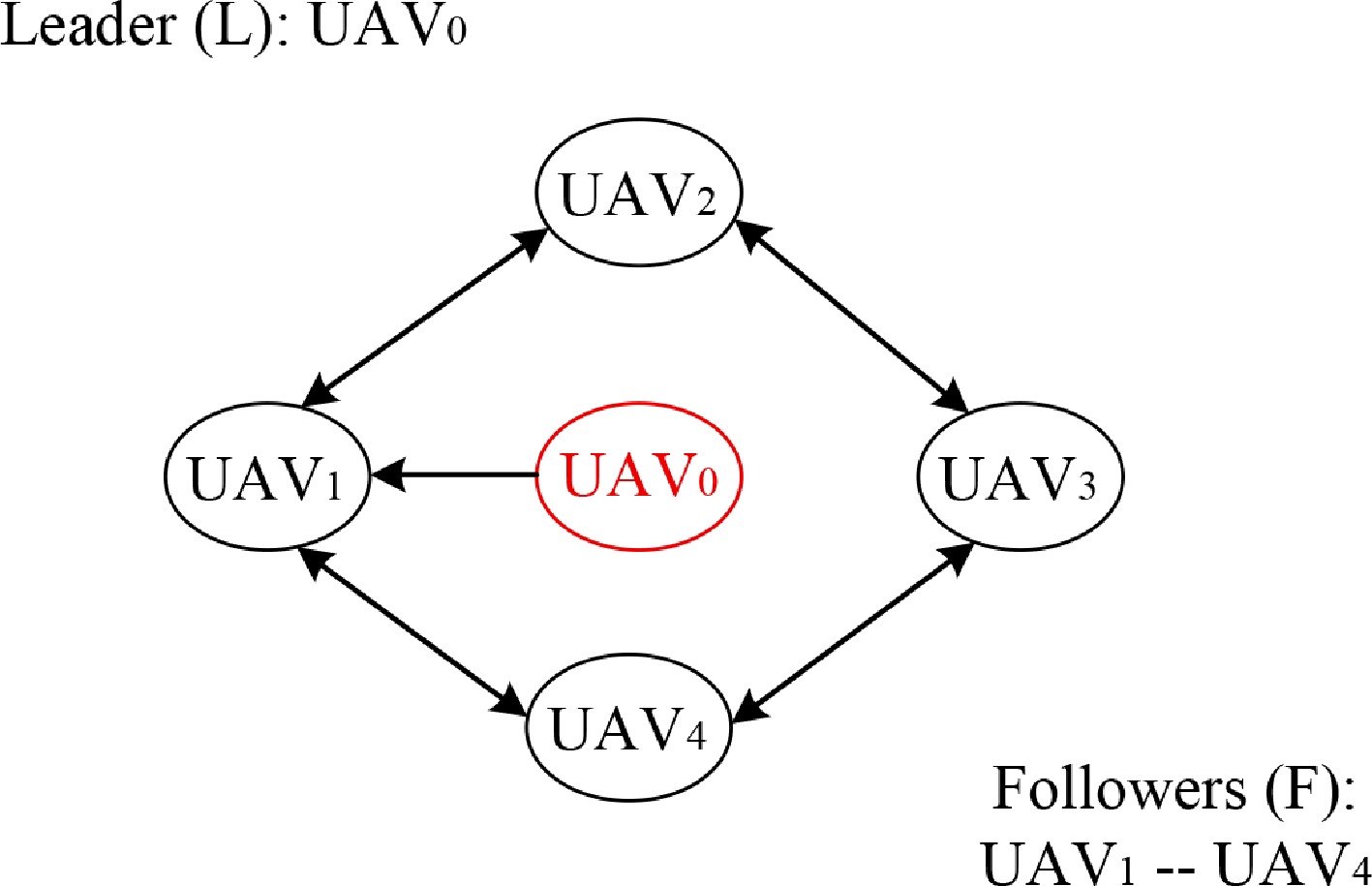
Figure 3. 

MUAVS communication topology schematic diagram.

The reference position of the leader UAV is $ {\ell _d} = [0.1{t^2},0.1{t^2},0.1{t^2}]$, the parameters of each follower UAV are $ {{\lambda _{\ell i}} = diag\left\{ {3,3,8} \right\}} $, $ {\lambda _{\varsigma i}} = { diag\left\{ {5,5,7} \right\}} $, i = 1, 2, 3, 4. Their relative positions are illustrated in Table 1.

According to (8), the parameters of the exogenous system is given as

The other control design parameters are chosen as

The simulation results are displayed in Figs 4−11. Figure 4 exhibits the disturbance estimation, where orange and green dashed lines represent the estimated upper and lower bounds, while the black solid lines are the actual disturbance values. Simulation results demonstrate that the designed IDO can cover the disturbance estimate at any time, rather than only after the estimation error has converged. This also implies an improved disturbance rejection capability of the MUAVS throughout the entire process.

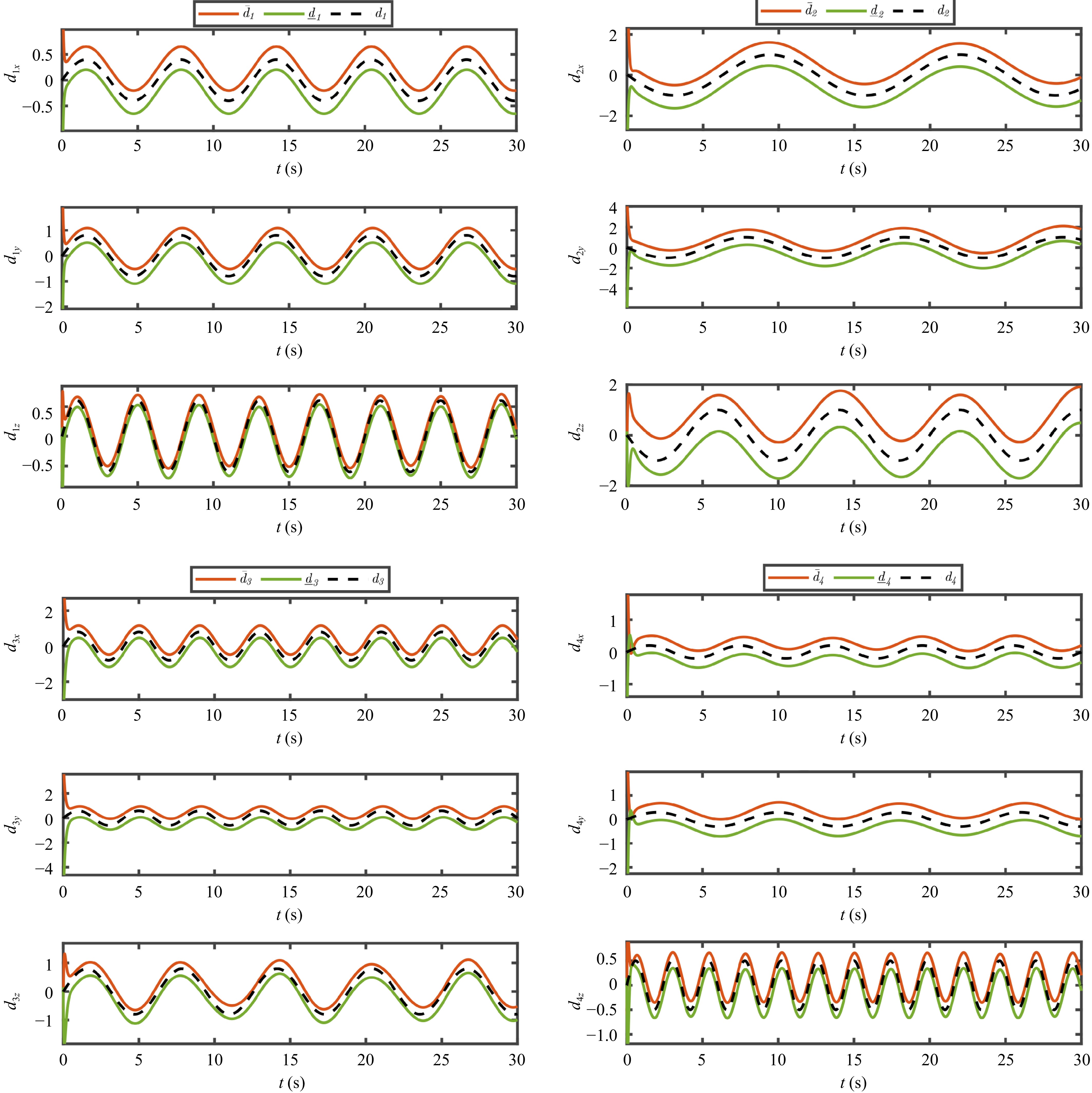
Figure 4. 

Estimation results of unknown disturbance under the IDO.

Moreover, comparative simulations are performed to validate the superiority of the designed IDO compared with the traditional ESO. The mean value of the upper and lower bounds of the IDO is adopted as the disturbance estimation. Figure 5 presents these comparative results, where the black dashed line represents the actual disturbance, the blue dashed line denotes the estimated result of the ESO, and the orange dashed line is that under the proposed IDO. As evident from Fig. 5, both the IDO and ESO methods are capable of accurately estimating unknown disturbances. However, unlike the ESO, which requires a finite convergence time to asymptotically track the disturbance, the proposed IDO provides mathematically guaranteed upper and lower bounds from the very initial moment. Furthermore, the IDO achieves smaller overshoot and a faster transient response.

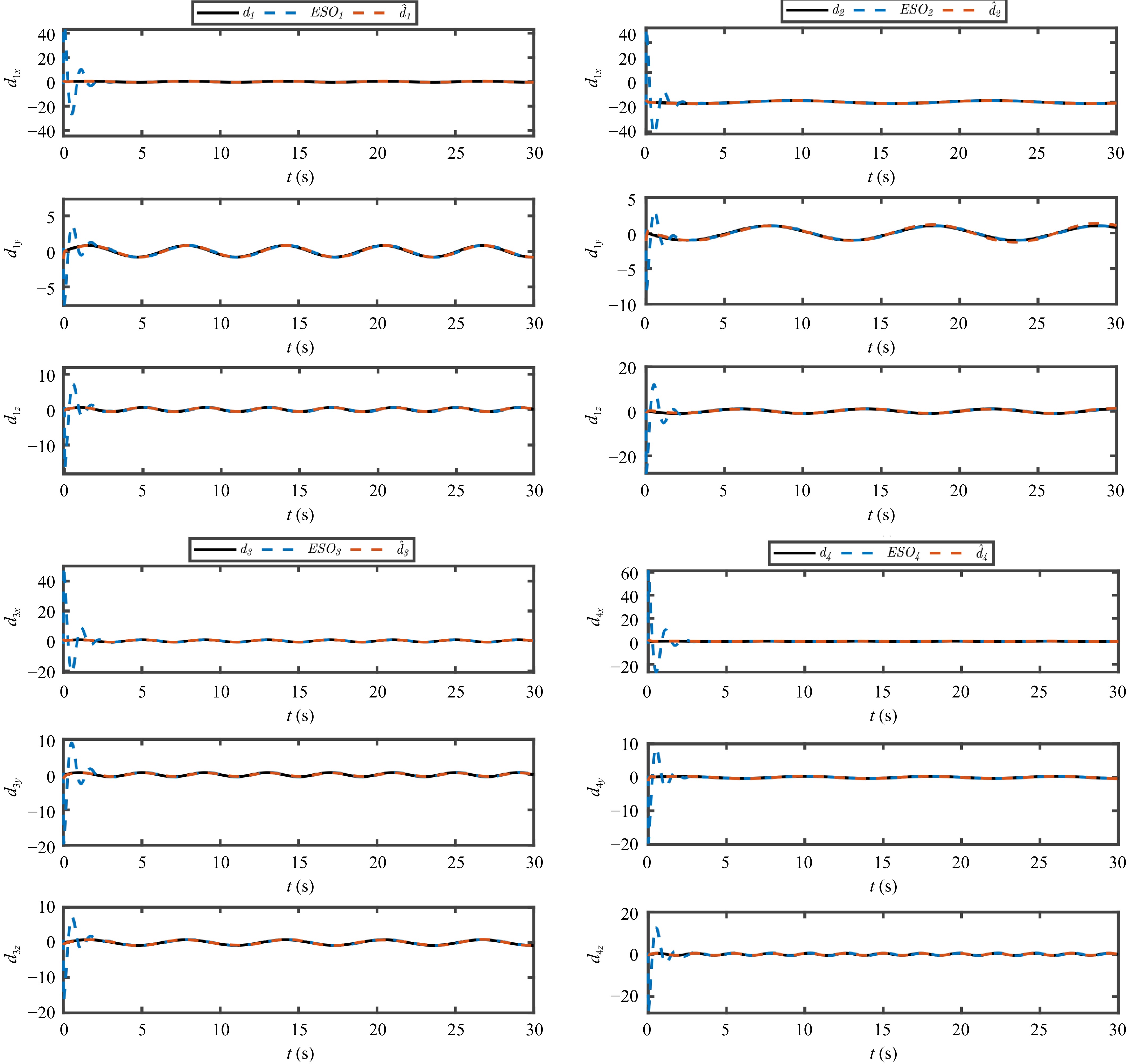
Figure 5. 

Comparison of estimation results of unknown disturbance under the IDO and ESO.

Meanwhile, to verify the feasibility and advantage of the proposed CBF-based obstacle avoidance strategy, comparative simulations against the conventional artificial potential field (APF) method are performed. In the APF paradigm, the destination generates an attractive potential acting on the UAV, while each obstacle produces a repulsive potential. The resultant force is the vector superposition of the attractive force from the destination and the repulsive forces from all obstacles, and the UAV reaches the target when its potential energy drops to zero. It is well recognized, however, that the APF approach suffers from intrinsic limitations, notably the goal non-reachability and local minima issues.

To illustrate the non-reachability problem, we place an obstacle near the target at coordinates (100,100,100), as detailed in Table 2. This obstacle, denoted as Obstacle$ _5 $, lies closest to the destination and falls within the attractive influence region of the UAV$ _1 $. As a result, when the UAV approaches the target, the repulsive force from the obstacle overwhelms the attractive force from the destination, leading to the well-known goal non-reachability phenomenon. As shown in Fig. 6, the UAV undergoes persistent oscillations in the vicinity of the target and ultimately fails to land on the desired point. By contrast, Fig. 7 reveals that under the proposed CBF-imposed constraints, the UAV reaches the target smoothly. These comparative results clearly demonstrate that the CBF method effectively overcomes the goal non-reachability defect inherent in the APF scheme.

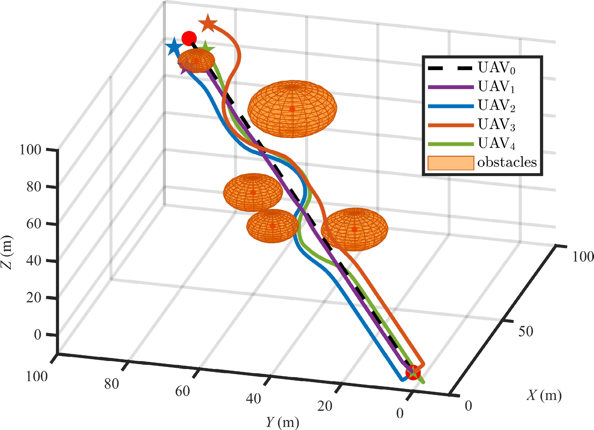
Figure 6. 

3D diagram of APF-based rectangular formation obstacle avoidance.

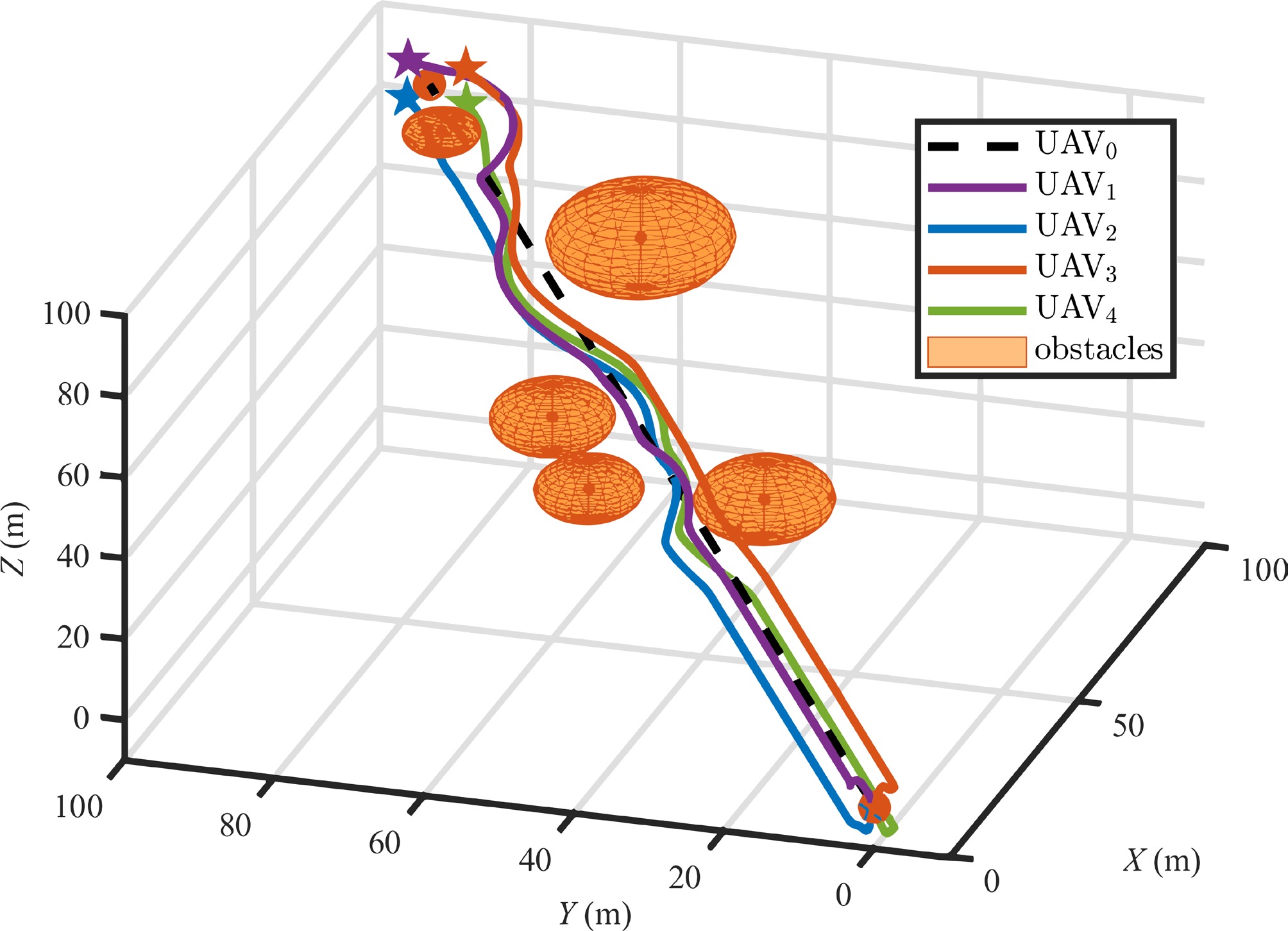
Figure 7. 

3D diagram of CBF-based rectangular formation obstacle avoidance.

The three-axis tracking trajectories and corresponding errors for UAV₃ and UAV₄ are depicted in Figs 8 and 9, where the dashed black line indicates the reference, and the orange and blue solid lines correspond to the CBF and APF schemes, respectively. Although both methods ensure collision-free navigation, CBF-QP yields less conservative safety adjustments, leading to shorter avoidance routes and tighter tracking with reduced position errors, as it formulates safety constraints in a mathematically optimized manner. With dynamically allocated control priority, formation control takes precedence in safe regions, whereas CBF-QP activates and enforces safety constraints upon obstacle proximity to guarantee strict safety distance margins.

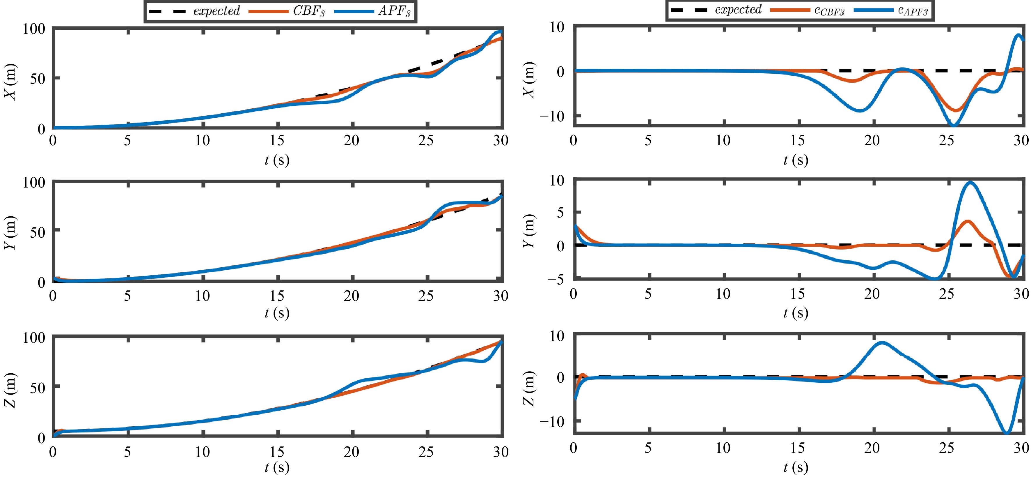
Figure 8. 

Comparison tracking results and error for UAV₃ under the CBF and APF.

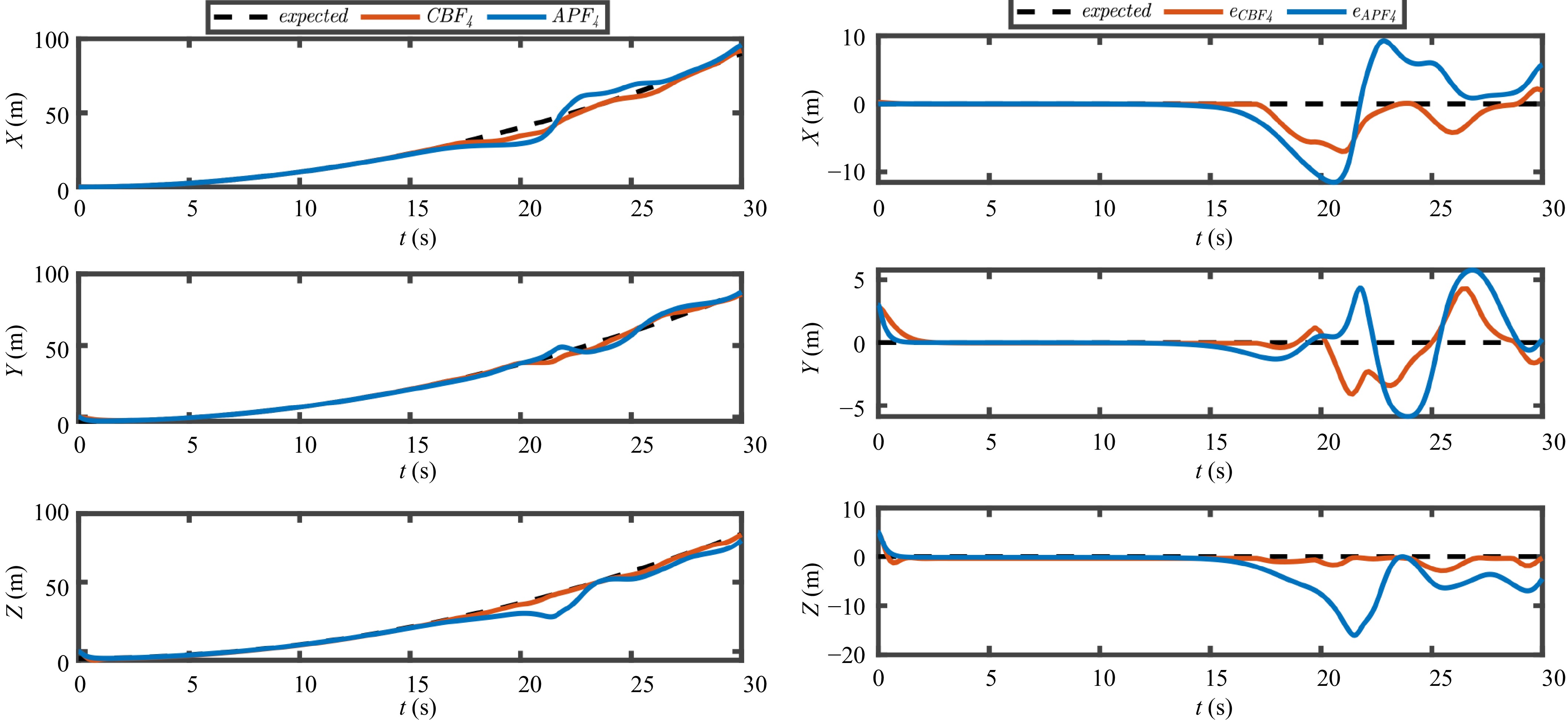
Figure 9. 

Comparison tracking results and error for UAV₄ under the CBF and APF.

This is further supported by the quantitative comparison in Tables 3 and 4, which list the MAE and RMSE for UAV₃ and UAV₄ during the obstacle-avoidance phase. The data consistently show that CBF offers smaller tracking errors and RMSE across most scenarios, along with more economical flight paths.

Figure 10 demonstrates the motion trajectories in three-dimensional coordinates under the CBF method, confirming that the formation reaches the predefined configuration within 5 s. When encountering obstacles, the UAVs maneuver to avoid them and quickly reconverge to the nominal formation path after passing. Figure 11 provides the time evolution of the flight-path azimuth angle, flight-path angle, and velocity for the four follower UAVs. All followers attain motion synchronization within 5 s. During obstacle avoidance, the states undergo noticeable transients. In particular, the velocity shows a clear deceleration phase when approaching obstacles, followed by a prompt acceleration phase to catch up and restore the commanded formation speed once the obstacles are bypassed.

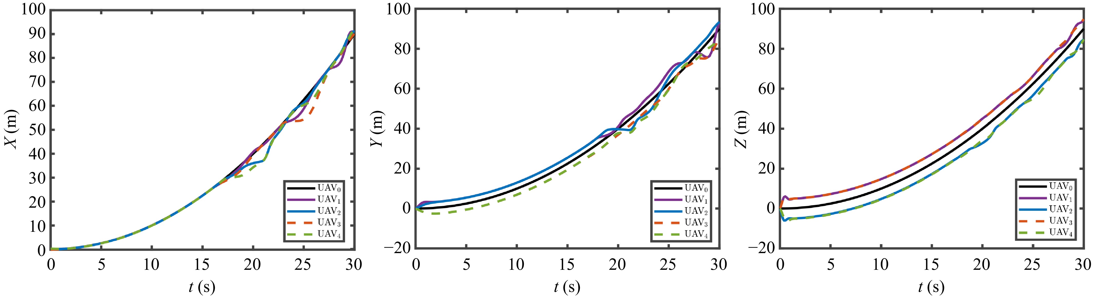
Figure 10. 

Three-axis position tracking of UAV formation.

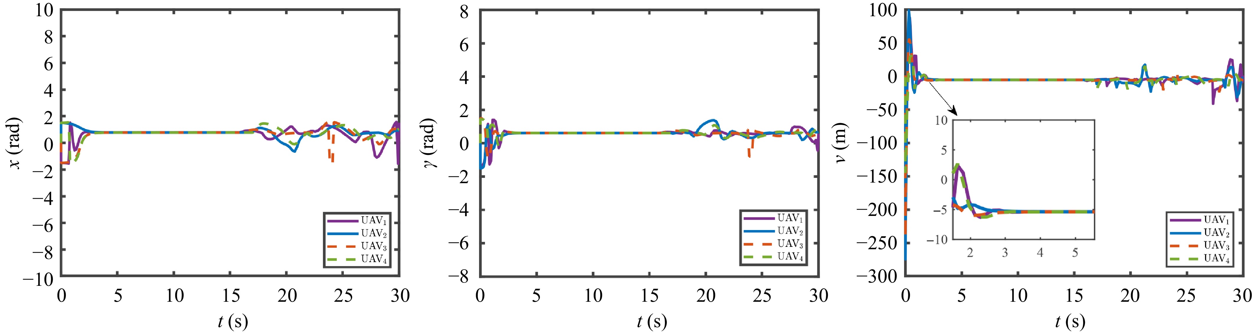
Figure 11. 

Flight path angles and speed of the UAV formation.

This work investigates the formation obstacle avoidance issue for MUAVS subject to unknown disturbances. Firstly, the fixed-wing UAV nonlinear dynamic equation is constructed, and the IDO is designed to suppress the adverse impacts of external disturbances on the system. Secondly, a consensus theory-based distributed formation control algorithm is developed to maintain the formation configuration. Meanwhile, to cope with environmental obstacles, a formation collision avoidance strategy is presented by integrating the CBF-QP technique. This strategy allows each UAV to perform timely obstacle avoidance maneuvers and rapidly restore the predefined formation configuration once obstacles are cleared. Finally, Lyapunov stability analysis is conducted to rigorously prove the uniform ultimate boundedness of all closed-loop signals, and numerical simulation results substantiate the superiority of the proposed method. In the future, the issues of real flight experiments, dynamic obstacles, and practical network communication constraints will be further explored in depth.