An integrated and cooperative architecture for multi-intersection traffic signal control

Urban traffic congestion has become a global issue and caused severe effects, such as increased travel time, fuel consumption, and air pollution^[1−3] It has serious implications for the global economy and the environment. For example, in recent years, the USA alone lost $87 billion per year in extra driving time and gasoline due to traffic jams^[4,5].

Inadequate traffic infrastructure, the rapid growth of vehicles, and pre-determined traffic signal control (TSC) methods are the leading causes of urban traffic congestion^[6]. Addressing urban planning and infrastructure concerns necessitates significant financial and material resources. As a result, improving the existing TSC methods is the most cost-efficient way to relieve traffic congestion.

In recent years, significant progress has been made on reinforcement learning (RL) for solving various sequential decision-making problems in Artificial Intelligence (AI) games, such as Atari^[7], Go^[8], and Dota2^[9,10]. The TSC problem can be regarded as an agent that can make decisions at intersections by interacting with the environment, just like in a game.

It is challenging to alleviate traffic congestion by optimizing and controlling traffic signals only at a single intersection^[11]. TSC is being extended from optimization of a single intersection to multiple intersections, which can be formulated as a multi-agent system with cooperation between agents. Hence, multi-agent reinforcement learning (MARL) has been receiving more attention from researchers in these years^[12−14]. Furthermore, considering the network transmission and communication between traffic lights, efforts toward efficiently deploying MARL in practice has remained a research challenge.

Additionally, most research focused on lab theories and algorithms with few considerations of industrial-scale deployment issues. With the limited capabilities of the network transmission bandwidth and underlying computing resources, optimizing the deployment structure and algorithmic performances for TSC is essential for intelligence transport systems (ITS).

ITS-related technologies, such as urban traffic simulation environments^[15−18], TSC algorithms^[19,20], and traffic signal communication^[14,21], have considerably enhanced traffic operation and management. To the best of our knowledge, there is rare research considering all aspects above for TSC, and few works can be deployed in the real-world. We summarize several existing challenges in TSC:

1) Although some studies have contributed to multi-intersection TSC^[22−24], it lacks an integrated architecture to leverage the traffic simulation environment, cooperative TSC algorithm, and traffic signal communication to achieve optimal multi-intersection TSC;

2) Traditional algorithms in urban TSC rarely consider traffic light cooperation and communication simultaneously;

3) Most studies optimize the algorithms but ignore the network capacity or latency in the urban TSC process.

To address the aforementioned challenges, an integrated and cooperative architecture for TSC across multiple intersections is proposed in this paper. The main contribution is threefold:

1) An integrated architecture, namely General City Traffic Computing System (GCTCS), is proposed, which integrates an urban traffic simulation environment, TSC algorithm, and communication across the traffic signal network simultaneously.

2) A MARL algorithm, namely General-MARL, is developed for TSC based on GCTCS, considering cooperation and communication between traffic lights.

3) Comprehensive experiments have been conducted to validate the proposed architecture and algorithm with promising results. From experimental results, our novel architecture is much closer to the real-life traffic environment. With the proposed algorithm, the average speed of vehicles is increased by 23.2%, and the network latency is reduced by 11.7% compared with baseline algorithms.

The remainder of this paper is organized as follows: Section Related Work introduces related works. Section Preliminary explains the basic concepts and problem definition. Section Methodology describes the architecture of GCTCS and details the General-MARL method for cooperative traffic light control based on GCTCS. Section Experiments conducts experiments to demonstrate the advantage of the General-MARL algorithm. Section Conclusions concludes the paper and discusses future work.

In this section, we discuss and introduce studies on the TSC, which can be divided into two typical categories: Conventional approaches and RL-based methods.

Conventional methods for TSC

Conventional TSC methods are classified into four types: fixed-time control^[25], actuated control^[26], adaptive control^[27], and optimization-based control^[28]. Fixed-time is a conventional and primary method of urban TSC, benefiting from the simplicity of deployment. It usually consists of a pre-timed cycle length, fixed cycle-based phase sequence, and phase split. While calculating the cycle length and phase split, the traffic flow is assumed to be uniform during a specific period. Since introduction in the 1950s^[25], it has been a leading solution to TSC in practice considering that the urban traffic environment is complex and uncertain, and mathematical approaches cannot precisely build a model from internal operational mechanisms of a TSC system. Actuated control^[26] decided whether to keep or change the current phase based on the pre-defined rules and real-time traffic data. It could set the green signal for a specific traffic signal phase if the number of approaching vehicles is larger than a threshold. Based on traffic volume data from loop sensors, adaptive control^[27] created a set of traffic plans and chose the one that was best for the current traffic situation. Optimization-based control^[28] formulated TSC as an optimization problem under a dynamic traffic flow and decided the traffic signal according to the observed traffic information. All of the methods discussed above heavily rely on human-designed traffic signal plans or rules.

RL based methods for TSC

RL-based methods have emerged as a promising TSC solution, which are designed for different application scenarios including single intersection control^[11,29], and multi-intersection control^[30,31].

Single intersection control

Abdulhai et al. ^[11] introduced Q-learning for TSC and presented a case study involving application to traffic signal control. Li & Wang^[29] proposed the idea to set up a deep neural network (DNN) to learn the Q-function of reinforcement learning from the sampled traffic state/control inputs and the corresponding traffic system performance result. Park et al.^[32] developed two traffic signal control models using reinforcement learning and a microscopic simulation-based evaluation for an isolated intersection. Additionally, the models could also be adapted for two coordinated intersections.

Multi intersection control

Multi-agent reinforcement learning (MARL) involves the participation of more than one agent^[12]. It can learn through the cooperation of (1) sharing instantaneous information through interaction with the environment and (2) sharing learned policies in episodic experience.

MARL is a suitable method for the TSC problem, which can be solved as a typical MARL system for optimization of all intersections^[13,14]. There exist intelligent traffic agents in the environment that can facilitate learning progress in MARL. Co-DQL model^[12] used a highly scalable independent double Q-learning method based on double estimators and the upper confidence bound (UCB) policy for multi intersections. Wang et al.^[13] proposed two distributed MARL control models as well as a Federated Learning (FL) framework to solve the ATSC problem, where the former is based on Advantage Actor-Critic (A2C) algorithm, and the latter is based on Federated Averaging (FedAvg) algorithm. El-Tantawy et al.^[30] investigated the following dimensions of the control problem: (1) RL learning methods, (2) traffic state representations, (3) action selection methods, (4) traffic signal phasing schemes, (5) reward definitions, and (6) variability of flow arrivals to the intersection. Rasheed et al.^[31] designed a multi-agent DQN (MADQN) and investigated its use to further address the curse of dimensionality under traffic network scenarios with high traffic volume and disturbances. El-Tantawy et al.^[30] introduced a multi-agent auto communication (MAAC) algorithm, which is an innovative adaptive global traffic light control method based on multi-agent reinforcement learning (MARL) and an auto communication protocol in edge computing architecture. The MAAC model considered traffic communication but did not leverage MARL and traffic simulation environment optimization.

From the literature, we find that most studies attempt to develop an RL or MARL model to address the TSC problem directly, ignoring the traffic simulation environment optimization and traffic communication simultaneously.

In order to create models for simulating complex traffic dynamics, urban traffic simulation systems typically integrate computing technologies and operational features of traffic flow (as illustrated in Fig. 1). Road network, vehicle description, traffic signal control, and communication between the simulation system and traffic equipment are typically the basic elements of an urban traffic simulation system.

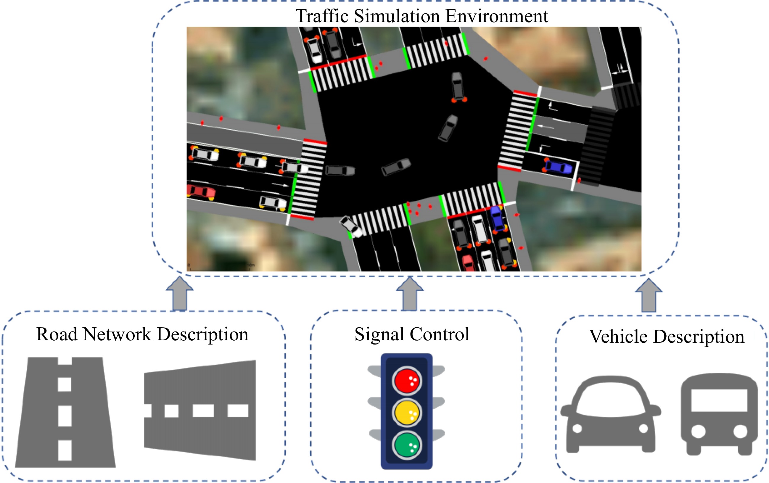
Figure 1. 

An urban traffic simulation environment for traffic research.

The traffic simulation system can be divided into two groups: the commercial and open-source system. VISSIM^[33] and Paramics^[34] are widely used as commercial traffic simulation systems. While, open-source systems, such as MIT Simlab^[15], SUMO^[16], CityFLow^[17] are usually adopted by researchers.

Traffic computing structure

Communication is one of the key functions in cooperation, which usually suffers from inevitable network latency. However, relevant studies on the development and deployment of computing frameworks often ignore the network delay in communication. In general, there are three major IoT computing structures, namely cloud computing^[35], fog computing^[21], and edge computing^[36].

Cloud computing is a ubiquitous, convenient, and on-demand repository of computing resources such as networks, servers, and storage. Fog computing is closer to where data is generated than cloud computing. Edge computing and data processing are performed at the nearest location where terminal devices generate the data.

Problem definition

The TSC problem can be regarded as an agent that can make decisions at intersections by interacting with the environment.

It can be formulated as an Markov Decision Process (MDP)^[37] ($ \left\langle{S,A,P,R,\pi ,\gamma }\right\rangle $), with the traffic state set S, action set A, transition probability P, reward R, control policy $ \pi $ and discount factor $ \gamma \in \left[\mathrm{0,1}\right] $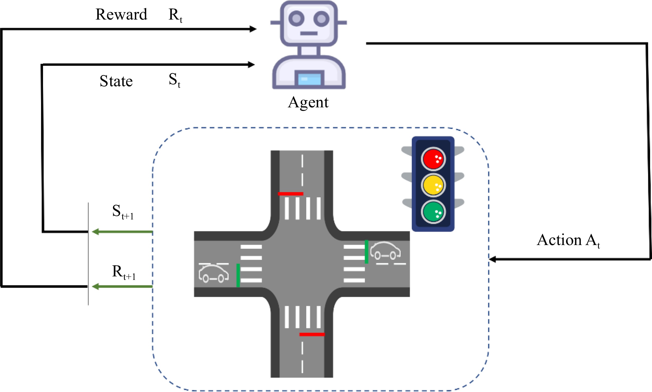, as shown in Fig. 2.

Figure 2. 

An illustration of traffic signal control at an intersection. According to the current traffic state $ {S}_{t} $ and the reward $ {R}_{t} $, the agent selects and executes the corresponding action $ {A}_{t} $ (change or maintain the current traffic light). Then the agent evaluates the effects of the action to obtain a new traffic state $ {S}_{t+l} $ and a new reward $ {R}_{t+1} $.

In this paper, we formalize the TSC problem as decentralized intersection optimization by MARL for multi-intersection (as shown in Fig. 3). Each intersection $ {I}_{i} $ is controlled b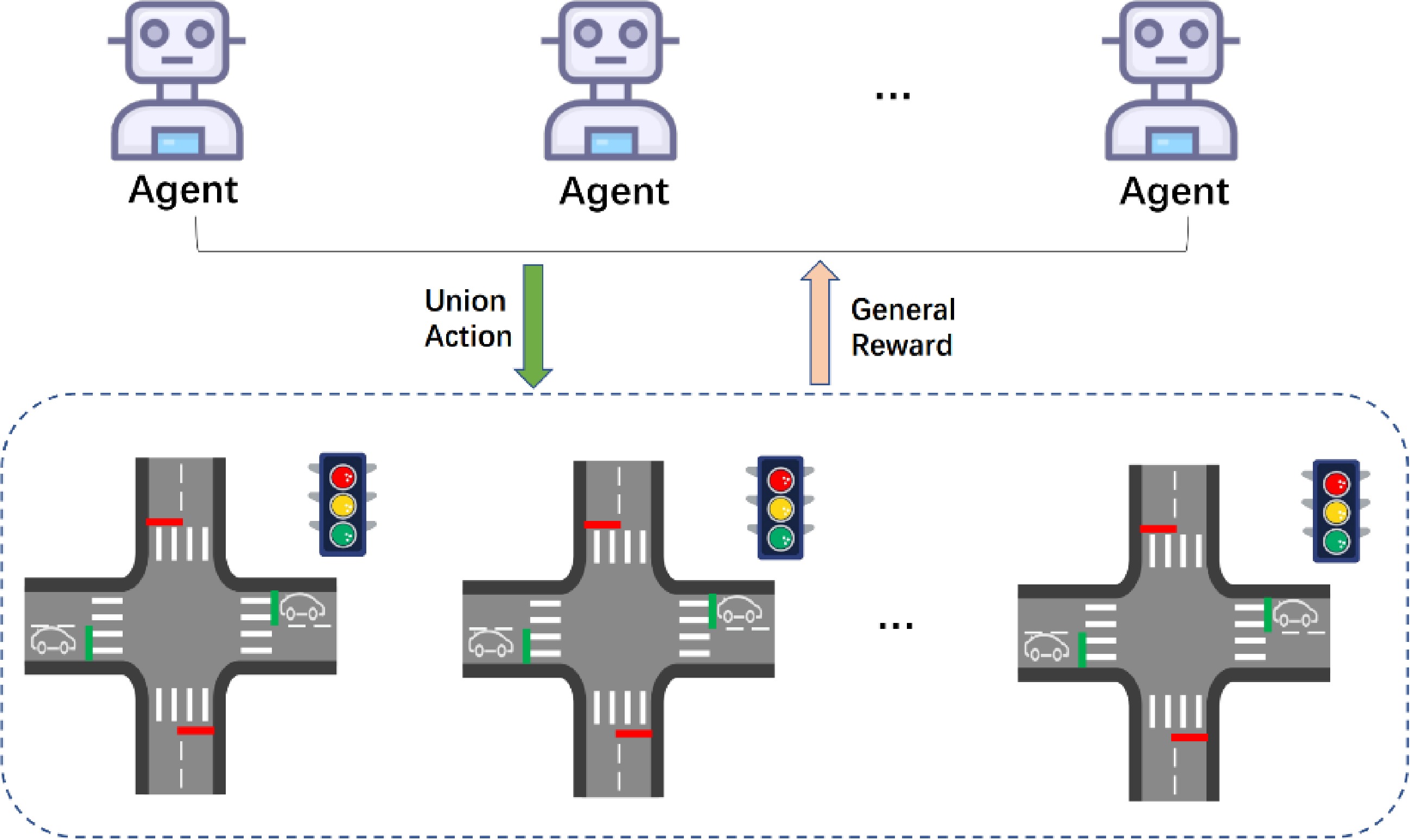y an algorithm $ {A}_{i} $. At time step $ t $, $ {A}_{i} $ makes an optimal decision to choose proper signal phase after analyzing its observation of the traffic state $ {\mathrm{S}}_{i} $ (vehicle queue, number of vehicle and etc.) at the intersection. In this case, the time T (average travel time) that vehicles spend in the traffic network can be minimized, denoted as:

Figure 3. 

The MARL structure in urban traffic signal control.

where $ {T}_{i}^{{I}_{i}\left({A}_{i}\right({\mathrm{S}}_{i}\left)\right)} $ is the average time vehicles spending at intersection $ {I}_{i} $ based on algorithm $ {A}_{i} $ on state $ {\mathrm{S}}_{i} $.

In a multi-agent system, the cooperation between agents is usually based on one computing structure. Thus, an effective and efficient integration solution covering different aspects is needed for TSC in practice.

In this section, we introduce an integrated and cooperative architecture, i.e., GCTCS, for urban TSC across multiple intersections. It integrates an urban simulation environment, a hybrid computing framework (cloud computing, fog computing, and edge computing), an interface for TSC algorithm deployment, a dynamic prediction module of traffic flow for traffic configuration interface, and an edge computing node of real-time traffic video processing^[38].

The development of GCTCS is to support more synthetic and efficient TSC experiments involving multiple intersections and to provide simulation data that are closer to real traffic conditions for industrial deployment, as shown in Fig. 4.

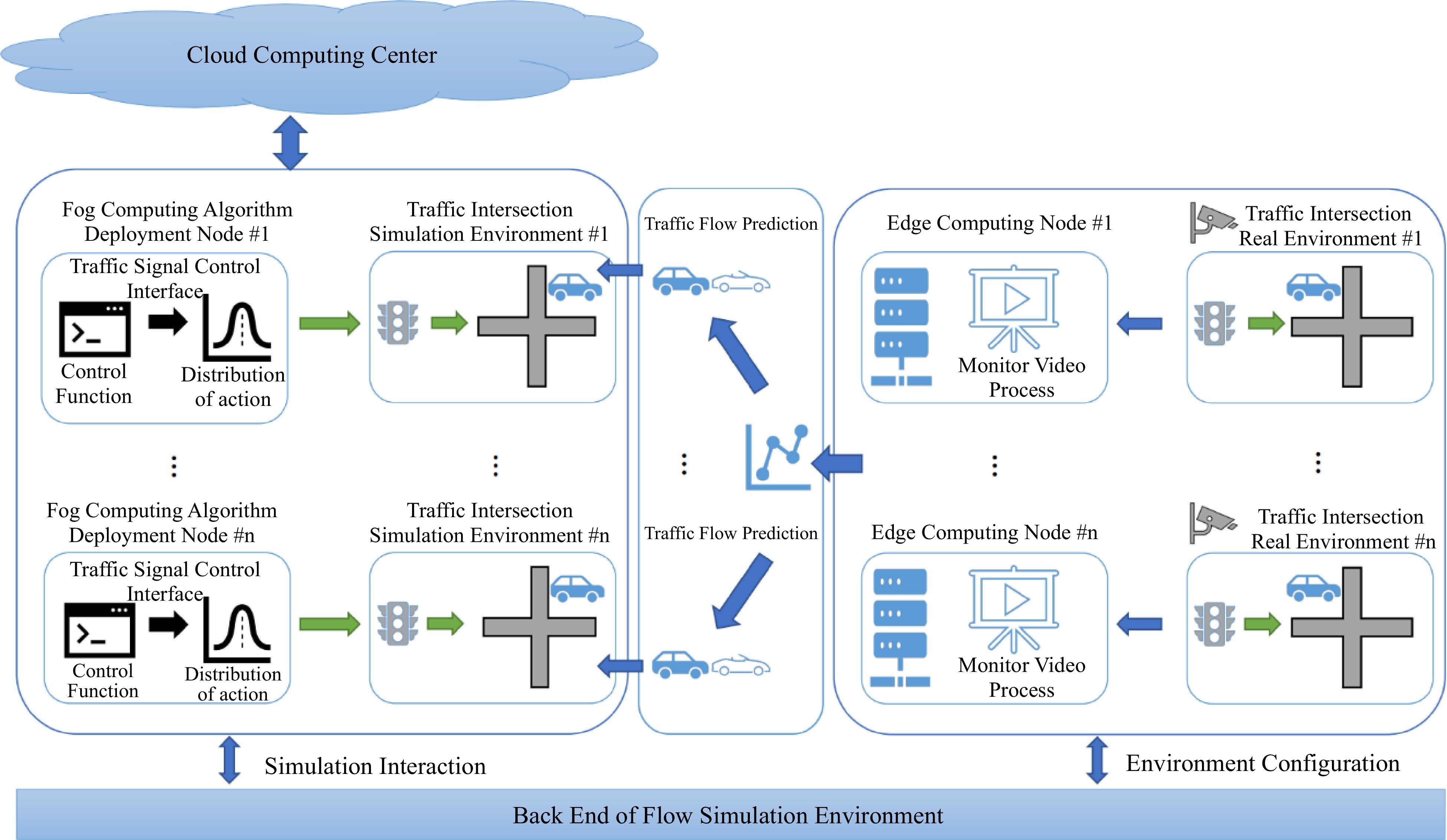
Figure 4. 

The General City Traffic Computing System (GCTCS) for urban traffic signal control.

GCTCS dynamically connects the simulation environment with the natural environment of multi-intersection traffic signals; provides urban TSC algorithm interfaces deployed under the hybrid computing architecture of cloud computing, fog computing, and edge computing; and takes complete account of network bandwidth and network delay. GCTCS can break through the barrier between the real traffic flow across multiple intersections and the traffic flow configuration of the simulation environment and realize dynamic synchronization between the real environment and the simulation environment. In addition, the overall computing architecture of GCTCS is based on a hybrid computing framework, which fully considers and simulates network delay. It provides interfaces for urban TSC and traffic flow prediction algorithms.

The functions of each layer

The cloud computing layer is located at the top layer of the architecture. It is responsible for interacting with each fog computing node in the fog layer, collecting information at the fog node, and sending control instructions from the cloud computing layer.

The fog computing layer is located between cloud computing and edge computing layers and consists of various powered servers, routers, and controllers that can bear heavy processing^[39]. The primary function is to compute and output the control signal instructions.

The edge computing nodes are located at the bottom layer, mainly processing surveillance videos and extracting status information at the current traffic intersection.

The module of traffic simulation environment

We designed the module of urban traffic simulation environment based on the urban traffic simulation platform described above, and it flexibly establishes the traffic flow forecasting interface for multiple intersections^[40]. The module can be configured by dynamic traffic flow based on the current simulation environment, making the environment more realistic.

This module employs the traffic flow forecasting method's external interface to dynamically construct traffic flow at each intersection, allowing the traffic simulation system to assimilate the current condition and provide an algorithm interface for TSC. The simulation environment FLOW framework^[18] is to optimize the urban traffic simulation environment benefiting from the forecasting capabilities based on data sets and time series models.

The traffic environments in different cities differ, and it is necessary to establish a unified method to obtain traffic circulating situations to construct the urban traffic environment closer to the real world (as shown in Fig. 5). The methodology (1) uses edge computing capabilities to convert the traffic flow captured in the urban traffic monitoring videos into text content; (2) applies a traffic flow prediction algorithm to predict relatively accurate traffic flow; and (3) dynamically interacts with the simulation environment's traffic flow configuration interface. The urban traffic environment is not built in isolation. It interacts with the simulation environment. The process is as follows:

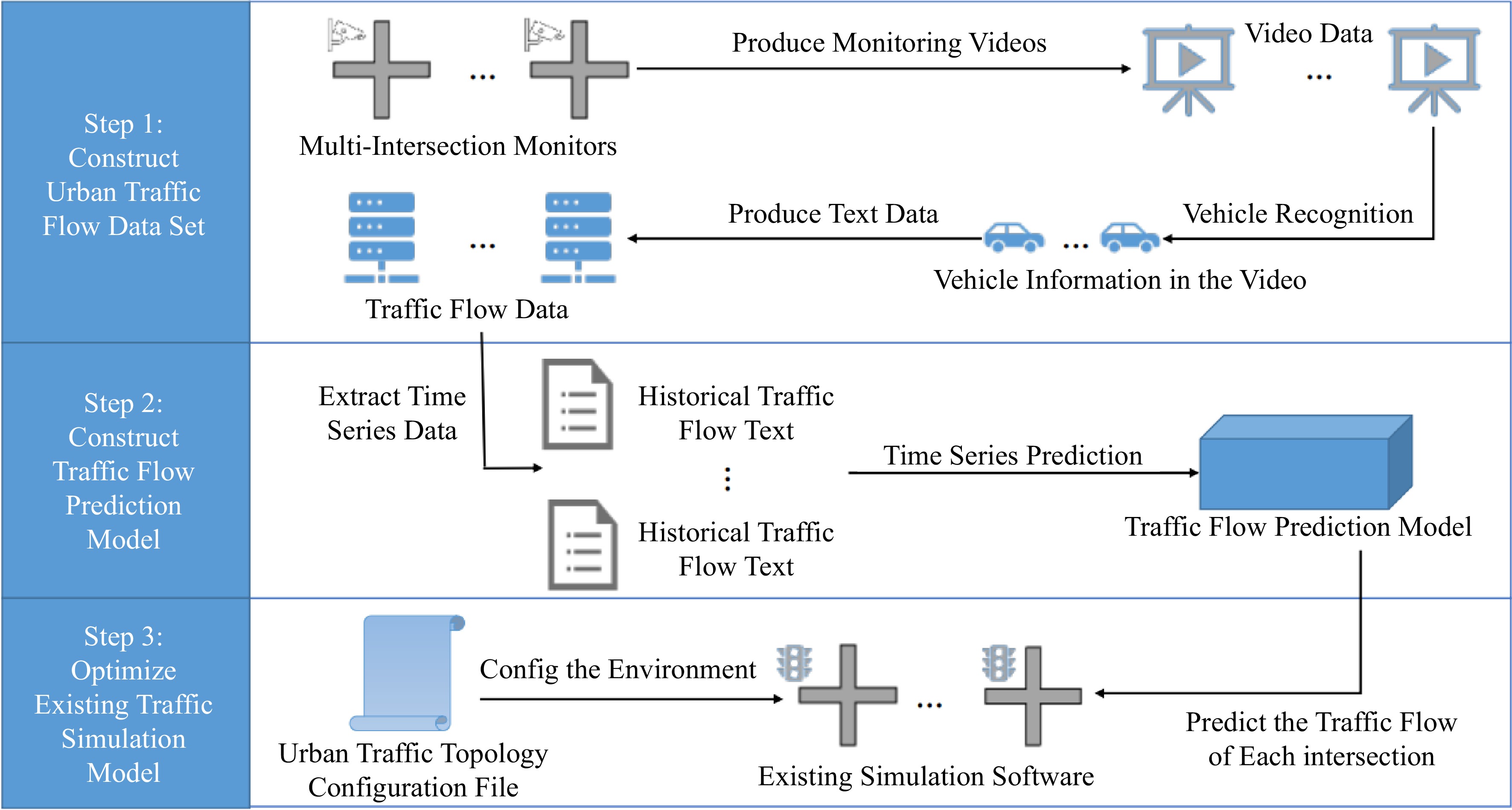
Figure 5. 

The processes of construction of the urban traffic real environment.

(1) Establish a data set of urban traffic flow;

(2) Design a forecasting model for traffic flow;

(3) Develop an interactive interface with the simulation environment.

The simulation environment interacts with the traffic flow anticipated by the traffic flow prediction model, allowing the simulation environment to configure real-time traffic flow.

General-MARL

In this section, we design a TSC method, named General-MARL, based on the GCTCS.

The design of the General-MARL algorithm is according to different layers of the GCTCS architecture. Thus, the General-MARL is composed of three sub-algorithms: the algorithm at the edge computing layer (Edge-General-control), the algorithm at the fog computing layer (Fog-General-control), and the algorithm at the cloud computing layer (Cloud-General-control). Additionally, the GCTCS with a layer-to-layer connection, which has a clear structure and lowers complexity compared to point-to-point connections, making feasible for the General-MARL with the increasing computation ability for edge and fog devices.

The Cloud-General-control produces the global control signal for each fog node's parameter updating based on the joint state (all traffic states from each node) and playback mechanism (historical interactions from fog nodes). The Fog-General-control generates a TSC signal according to the traffic state abstraction from Edge-General-control, the intelligent communication between agents allows an agent to share the learned strategies and the parameters from the cloud layer. Deep neural networks^[41] are the basic component in General-MARL for generating control actions, communication information, and so on. The structure of the algorithm architecture is illustrated in Fig. 6.

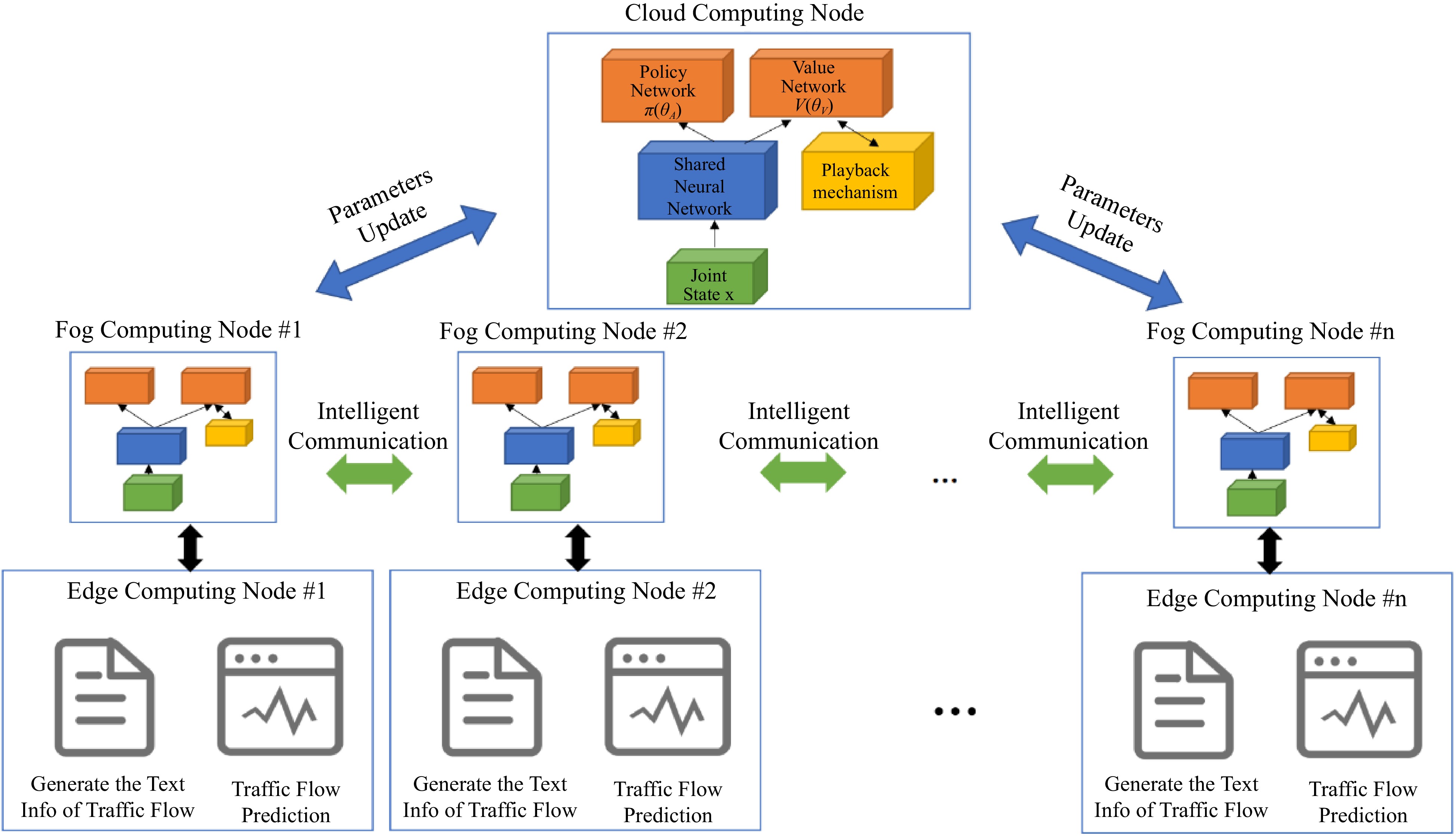
Figure 6. 

The General-MARL is composed of three sub-algorithms based on different layers of the GCTCS architecture.

Edge-General-control

The Edge-General-control algorithm processes the traffic surveillance video based on the target detection algorithm YOLO^[38], detecting the vehicles' location at the intersection.

As shown in Fig. 7, we apply an open-source vehicle image dataset, i.e., BIT-Vehicle^[42], to fine-tune the YOLO algorithm for vehicle detection precisely. The center of each intersection is the center point (0,0). We get the vehicle position from the YOLO-based model and add two fully-connection (FC) layers for fine-tuning. Then, we obtain the direction information according to the vehicle's location and center position. Hence, traffic state text is abstracted from the traffic surveillance video, including the vehicle-id, type, direction, and timestamp for passing vehicles.

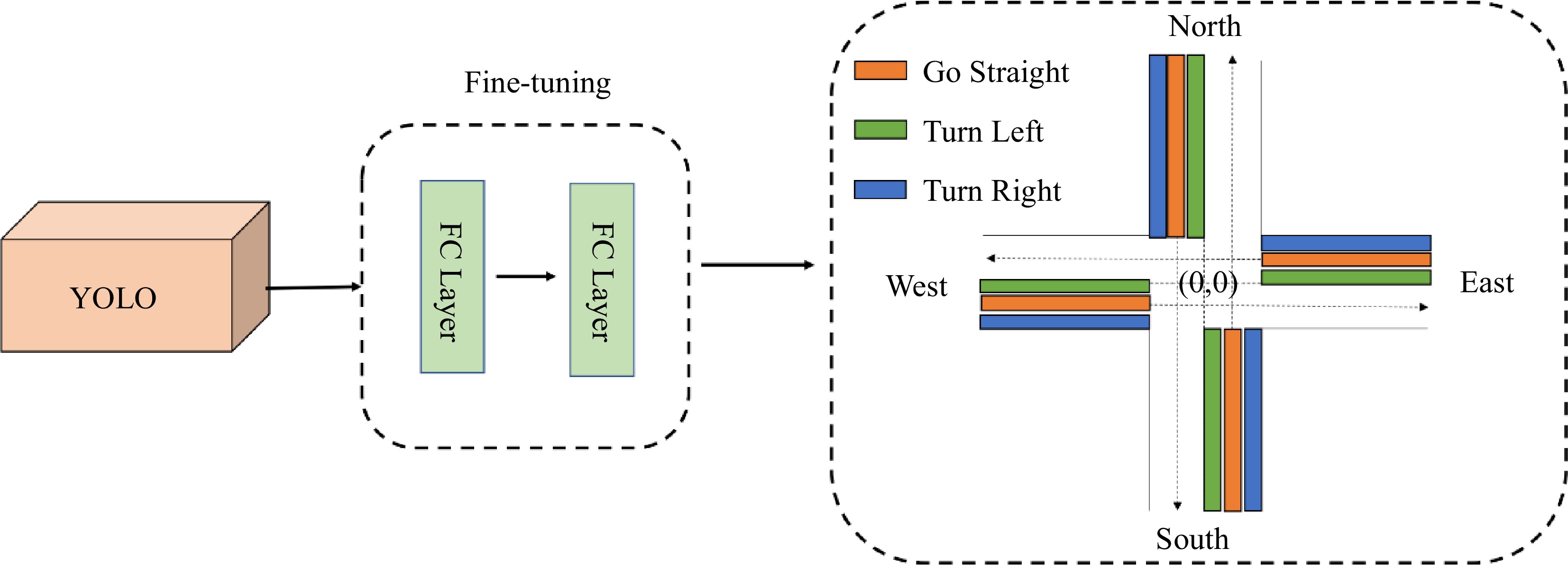
Figure 7. 

The process of abstracting traffic information from the video to generate the text info from traffic flow. Detection of vehicles in the three regions stands for different directions of passing vehicles

Finally, we introduce the traffic flow prediction algorithm GCN-GAN^[40], which can predict the traffic flow and synchronizes with the simulation environment in real-time (Algorithm 1).

Fog-General-control

The Fog-General-control algorithm includes the Nash-MARL module and the communication module to generate control strategies for urban traffic signals.

Nash-MARL Module: The Nash-MARL Module is to obtain Nash equilibrium for TSC without prior knowledge dynamically^[43]. It defines that $ X $ is the traffic environment state space for multi-intersection; $ U $ is the joint action from agents to tune transfer signal; $ A $ is the action space of one agent $ a\in A $; joint action is $ {u}^{a}\in U $. $ R $ is the reward or objective function. The object of $ {Agent}^{i} $ is to choose a proper strategy $ {\pi }_{i} $ and to maximize the objective function $ {R}_{i} $.

Herein, the Bellman equation with Nash Equilibrium: firstly, fix other agents' policies $ {\pi }_{-i}^{*} $; optimize the objective function of $ {Agent}^{-i}:{R}_{i}\left(x;{\pi }_{i};{\pi }_{-i}^{*}\right) $:

Where $ {\pi }_{i}^{*} $ is $ {Agent}^{i} $' policy according to other agents' $ {Agent}^{-i} $ action selection policies. $ {\pi }_{i}^{*} $ and $ \gamma \in [0, 1] $. The result of the objective (reward) function is based on the policy selection for participated each agent. It automatically generates its action policy by considering the behavior of other agents. When the behavior of other agents is stable, $ {Agent}^{i} $ tries to optimize the behavior of the objective function. All agents' policies could achieve Nash equilibrium after iteration update.

In the design of the Nash-MARL Module, the computation of the critic function (advantage) in deep reinforcement learning might have positive (good) and negative (bad) reward results, making the learning process efficiently. Thus, the Nash-MARL module defines the $ Q $ function of an $ {Agent}^{-i} $ as $ {\left({\hat{Q}}_{i}^{\theta }\left(x;u\right)\right)}_{i\in N} $; the estimate value function of $ {Agent}^{-i} $ is $ {\left({\hat{V}}_{i}^{\theta }\left(x;u\right)\right)}_{i\in N} $, wherein $ u $ is the union action, and $ x $ is the union state.

It employs the actor-critic model^[44] as a framework. In the actor-critic model, the actor is a policy function and the critic is a value function. The parameter set $ \theta $ into the value function parameter set and the policy function parameter set $ \theta =\left({\theta }_{V},{\theta }_{A}\right) $, where $ {\theta }_{V} $ represents the model of the value function $ {\hat{V}}^{{\theta }_{V}} $; $ {\theta }_{A} $ represents the parameters of the agent (participant) action selection policy $ {\hat{\pi }}^{{\theta }_{A}} $. $ {x}_{m}^{\text{'}} $ is the next state of $ {x}_{m} $. The model samples M epochs. The object of the algorithm is to minimize the loss of the sampled data and the Nash-Bellman equation $ {L}_{m}\left(\theta \right) $:

The module defines $ {y}_{m}=\hat{L}\left(y,{\theta }_{V},{\theta }_{A}\right) $ for simplifying the above expression.

Inspired by the deep Q-networks^[7], the module also introduce a memory buffer (replay buffer) to store triples $ {y}_{t}=\left({x}_{t-1},u,{x}_{t}\right) $, which represents the previous state of the environment $ {x}_{t-1} $; the union operation performed $ u $; the next state of the environment $ {x}_{t} $; and the reward $ {y}_{t} $ that passes through this state. The module can use stochastic gradient descent (SGD) to update the parameters after randomly selecting a piece of memory data from the replay buffer. To improve the action plan, the algorithm also employs ϵ-greedy exploration.

Additionally, the idea of parallel space-time is incorporated to enable the simultaneous execution in various environments. To achieve a stable learning process, multiple explorations in multiple environments would explore different policies and accelerate the learning speed. The overall algorithm structure is shown in Fig. 6. Further, the Nash-MARL algorithm process is detailed in Algorithm 2.

Communication Module: The communication module between agents allows an agent to share the learned strategies with others based on the attention mechanism^[45].

The calculation steps in the communication module^[14] at time $ t $ are shown in Fig. 8. At a time $ t $ in the communication module, the environment input is $ {X}_{t}=\left({x}_{t}^{1},\cdots ,{x}_{t}^{N}\right) $ and the corresponding communication information input is $ {C}_{t}=\left({c}_{t}^{1},\cdots ,{c}_{t}^{N}\right) $. Multi-agents $ \left({Agent}_{1},\cdots ,{Agent}_{N}\right) $ are able to interact with each other. Each agent receives information from receivers and transmitters internally. The receiver receives its own environmental information $ {x}_{t} $ and communication information $ {c}_{t} $, and generates action and external interaction information group $ \left({a}_{t+1},{c}_{t+1}\right) $ at $ 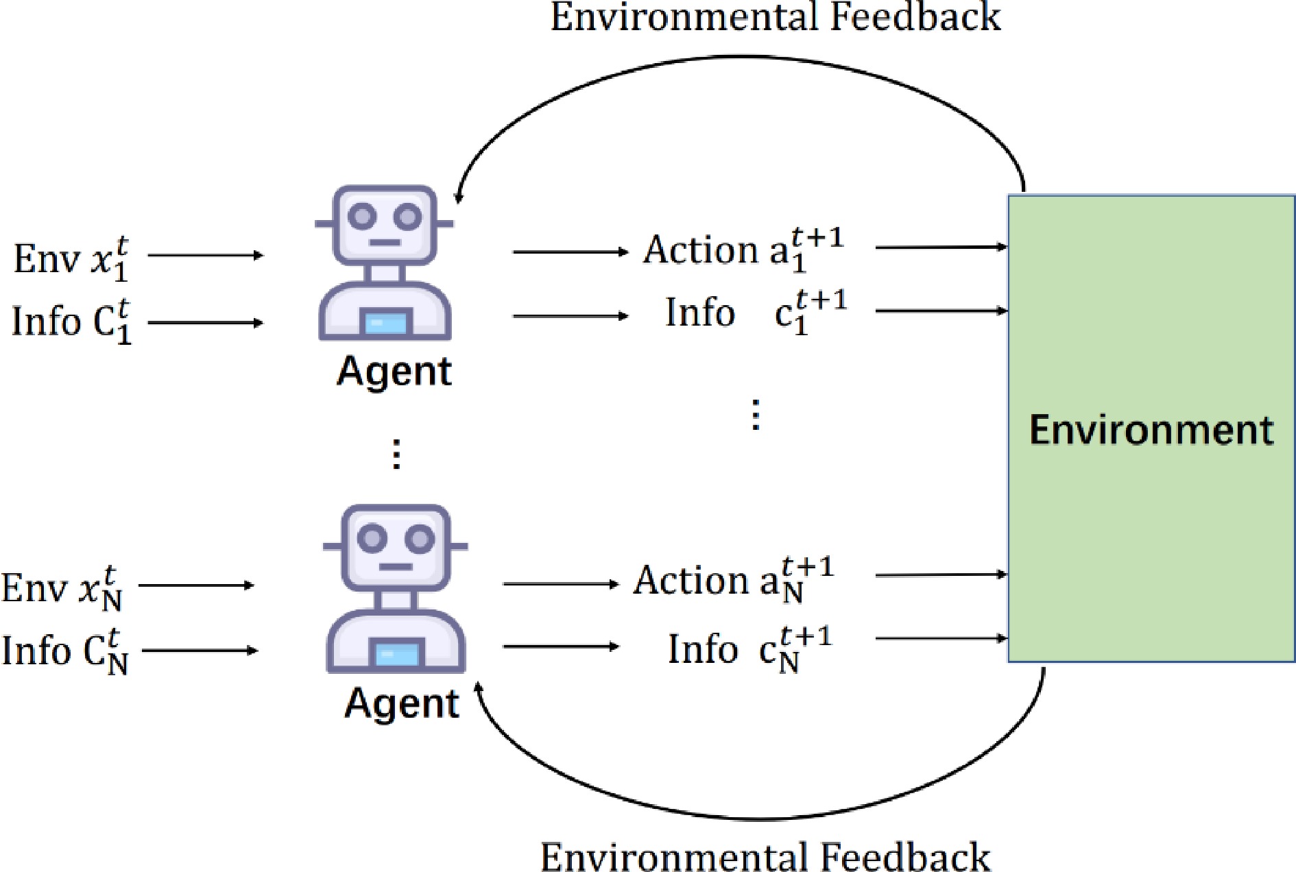t+1 $.

Figure 8. 

The communication process between agents in the communication module.

In the communication module (as shown in Algorithm 3), the parameter set of $ {Agent}^{i} $ for each agent is $ {\theta }^{i} $. Furthermore, $ {\theta }^{i} $ is divided into the sender $ {\theta }_{Sender}^{i} $ and receiver $ {\theta }_{Receiver}^{i} $. The parameters of the sending side and the receiving end are optimized by the overall multi-agent objective function. The parameter sets of the receiver and the sender are updated iteratively for each agent.

The Fog-General-control algorithm is illustrated as below (Algorithm 4):

Cloud-General-control

The Cloud-General-control algorithm deploys the Nash-MARL module, the 'parallel universe' of the Nash-MARL algorithm are fog nodes.

The Cloud-General-control Algorithm 5 is:

In this section, we apply General-MARL and baseline methods to the integrated and cooperative architecture GCTCS for multi-intersection TSC. The experimental process ignores or considers the situation of network bandwidth and network delay, respectively.

Dataset

The dataset from Lanzhou in China consists of two parts: (1) the traffic network; and (2) the traffic flow. The traffic network describes the traffic network, including lanes, roads, intersections, and signal phases. As shown in Fig. 9, there are 27 intersections connecting 45 roads. All the traffic networks are simulated in the simulation environment from our GCTCS. Various and flexible TSC algorithms control each intersection's signal. The distance between two intersections is two to four kilometers (km). The speed limitation is 60 (km/h).

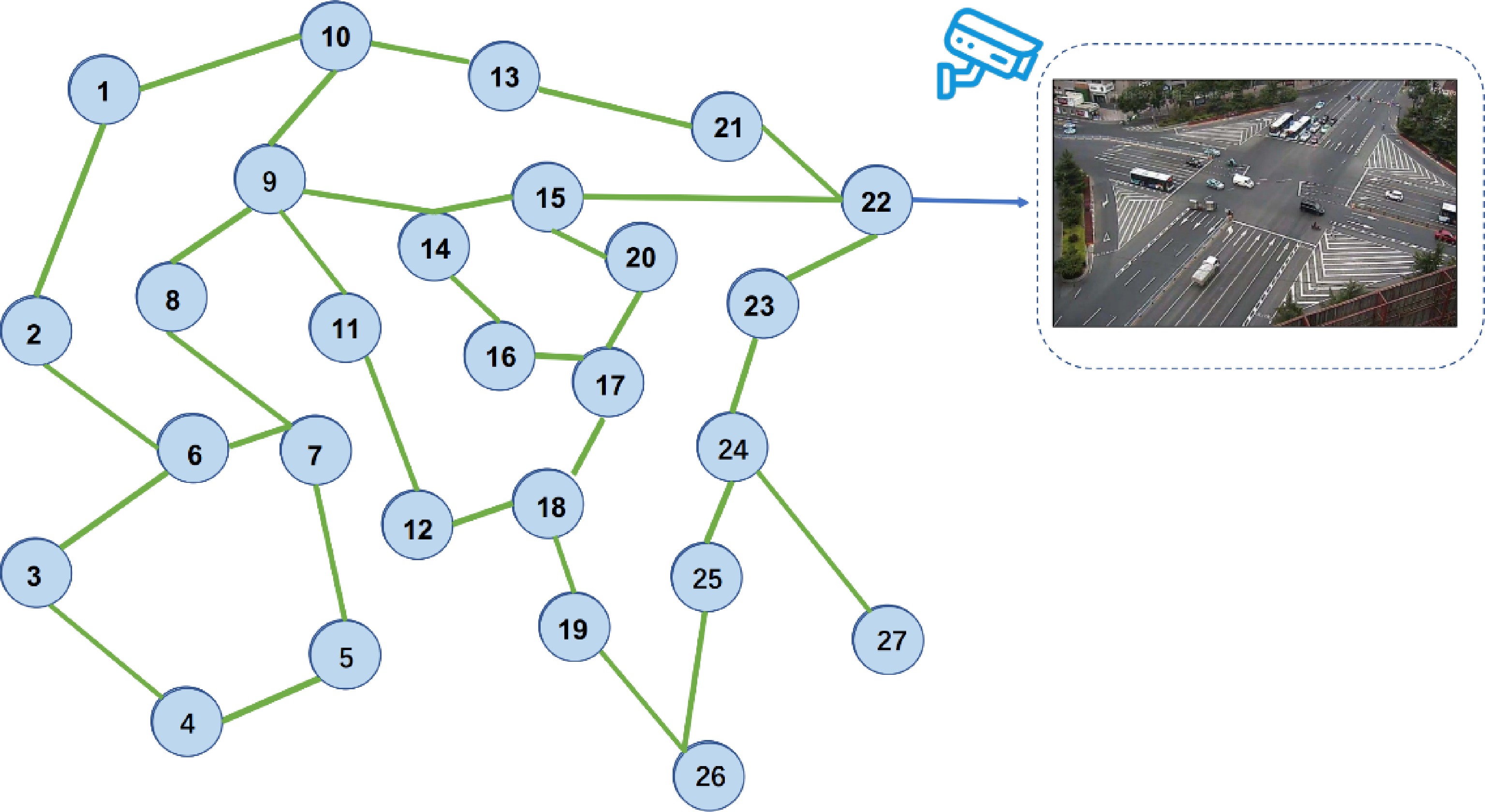
Figure 9. 

The illustration of topology map of real traffic intersection.

The initial flow of incoming and outgoing vehicles at each intersection is configured based on the real traffic flow data. The traffic flow dataset contains vehicles travel information, which is described as $ (t,u) $, where $ t $ is the time that each vehicle starts entering the traffic network and $ u $ is the pre-planned route from its original location to its destination.

Parameter settings of General-MARL

Cloud computing center

We deploy the Cloud-General-control algorithm in a Docker environment^[46], logically away from the intersections, and set the communication delay from the cloud center to the fog computing node to $ x $ seconds in the simulation code (set $x$ = 0 second to sleep to ignore network delay; set $x$ = 10 seconds to consider network delay). Then we set four hidden layers in the network for policy network generation $ \pi \left(x\right) $ in the cloud computing node with 40, 80, 80 and 80 nodes in each layer, respectively. The network layers are activated and connected through the activation function ReLU^[47]; the main neural network has three hidden layers, each containing 40 nodes. The layers are activated and connected through ReLU. The learning rate is set to 0.001.

Fog computing node

We deploy the Fog-General-control algorithm in the Docker environment and set it to be logically close to the intersection. The delay from the intersection to the fog computing node is set to $ x $ second (set $x$ = 0 second to sleep to ignore network delay; set $ x $ = 1 second to consider network delay). Twenty seven fog computing nodes are deployed in the environment. The network for policy network generation $ \pi \left(x\right) $ in each node is set with four hidden layers, with 40, 80, 80, and 40 nodes, respectively. The layers are connected through ReLU activation, and the main neural network has three hidden layers, each containing 40 nodes. The layers are connected through ReLU activation. The learning rate is set to 0.001.

Edge computing node

We deploy the Edge-General-Control algorithm in the Docker environment at one intersection. The network delay from the edge computing nodes to fog computing and vehicles are both set to $ x $ seconds (set $x$ = 0 second to sleep to ignore network delay; set $x$ = 1 second to consider network delay).

Initial traffic light period setting

The traffic control period is set to 60 s initially. The intervals of the green, red and yellow lights are set as ${g}_{t}$ = 27 s, $ {r}_{t} $ = 27 s, and $ {y}_{t} $ = 27 s, respectively.

Vehicle simulation

According to the actual traffic flow forecasting algorithm, the traffic flow is predicted every 15 min, and the vehicle simulation is conducted at each intersection.

Evaluation mechanism

In the simulation environment, the passing time of all vehicles at each intersection in an Episode is recorded as $ {T}_{e}={\sum }_{i=1}^{I}{\sum }_{m=1}^{M}{t}_{m} $, wherein $ e\in E $ is the number of Episodes, $ M $ is the number of vehicles, and $ I $ is the number of intersections. In this configuration, we set $E$ = 1,000; $ I $ = 27.

Methods for comparison

Fixed-Time^[25]: a policy gives a fixed cycle length with predefined green time among all phases. The intervals of the green, red and yellow signals are fixed as green and red are 27 s, and the yellow is 6 s, which are the same as the initial intervals for other methods for a fair comparison.

Q-learning^[32]: a model-free reinforcement learning algorithm to learn the value of an action in a particular traffic state based on Q-learning^[48], which leverages the advantage deep neural network for addressing TSC problem. The algorithm can be deployed on the Fog or Edge node with the same parameters as shown in Table 1.

Nash-Q^[49]: a model integrates Q-learning^[48] and Nash Equilibrium^[50] for making agents learn a better cooperative strategy, which can be deployed on the Fog node.

Nash-DQN^[51]: a Deep-Q-learning methodology for model-free learning of Nash Equilibrium for general-sum stochastic games.

MAAC^[14]: a multi-agent auto communication (MAAC) algorithm is an adaptive global TSC method based on MARL. MAAC combines multi-agent auto communication protocol with MARL, allowing an agent to communicate the learned strategies with others for achieving global optimization in traffic signal control. The intervals of the green, red and yellow signals are fixed as the experiment settings.

Experimental process

Each experiment consists of two parts: the first part ignores the network delay and compares results with other TSC algorithms; in the other part, network delay is considered.

Ignoring network delay

The delays of edge computing, fog computing, and cloud computing nodes in General-MARL are all set to 0 without considering network latency. In the urban simulation environment, we input actual traffic data before configuring various TSC algorithm models via the algorithm interface. Baseline methods and the General-MARL algorithm are run in the simulation environment. The traffic flow at each intersection is updated every 15 min. We record the waiting time of vehicles at each traffic intersection every minute (considered as an environmental feedback reward) and conduct 1000 Episode (round) training.

As shown in Fig. 10, the training convergence effect of the General-MARL algorithm is as good as the Nash-DQN algorithm but does not perform the best.

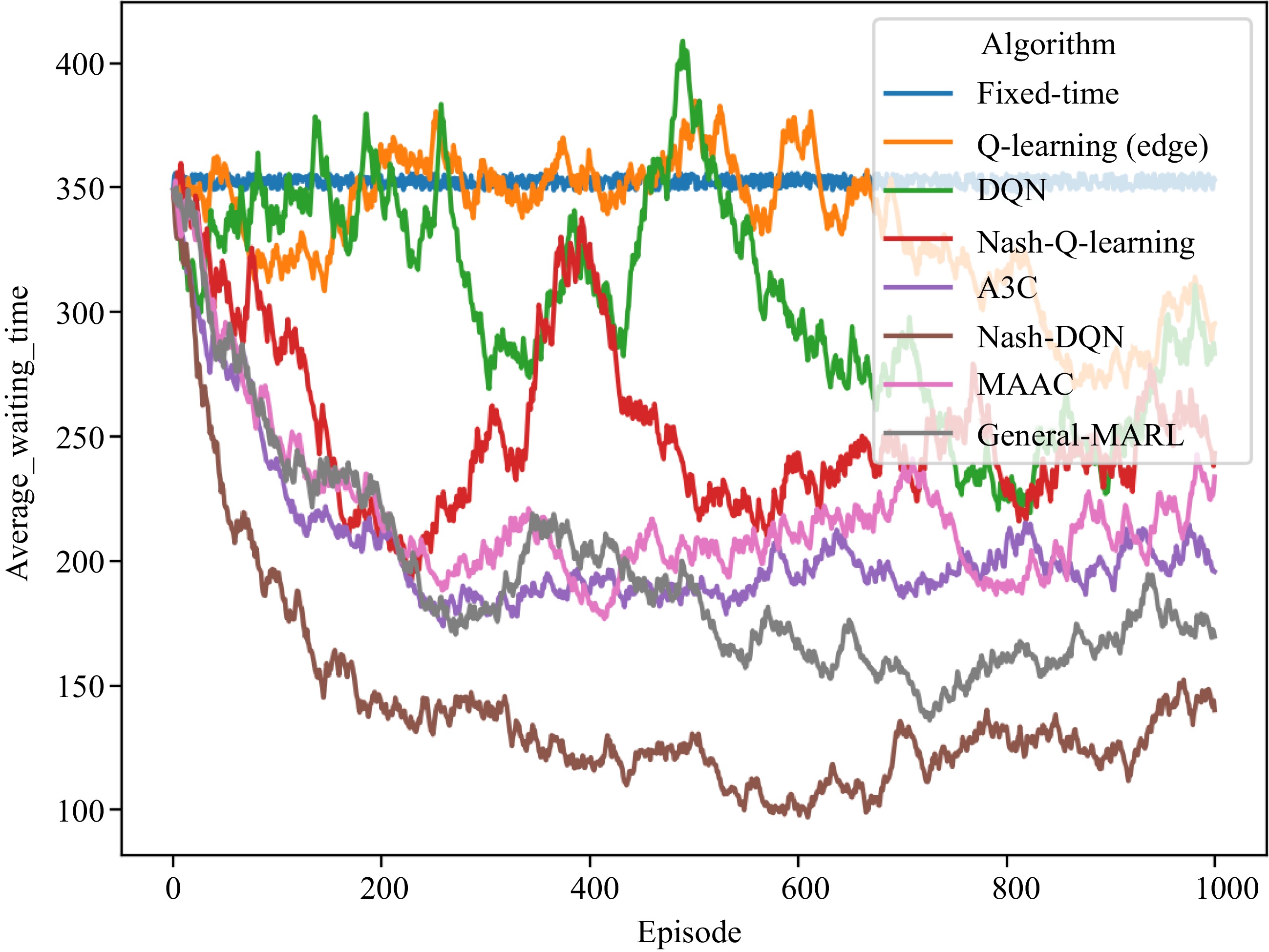
Figure 10. 

Multi-intersection traffic signal control training process (without network delay).

Considering network delay

In the case of considering network delay, the delays of the edge computing, fog computing, and cloud computing nodes in General-MARL are all set parameters according to the previous section. Then we configure the fixed duration as the traffic signal time series as the previous setting. Q-learning (edge) deploys the Q-learning algorithm on the fog computing node to control the traffic lights, and the delay from the controlling agent to the intersection is 1 s. There are 27 docker containers deployed at 27 traffic intersections with Q-learning capabilities to generate traffic flow controlling signals, respectively.

Q-learning (center) and DQN only use the cloud computing center to collect the information at each intersection. They are applied for overall control and generation of control commands for each intersection. The traffic flow prediction algorithm then updates the traffic flow at each intersection every 15 min (GCN-GAN). GCTCS records the waiting time of vehicles at each intersection every minute (as an environmental feedback reward) and conducts the training with 1000 Episodes.

As shown in Fig. 11, the convergence speed of the General-MARL is faster than Nash-DQN, and the training results outperform other baseline algorithms.

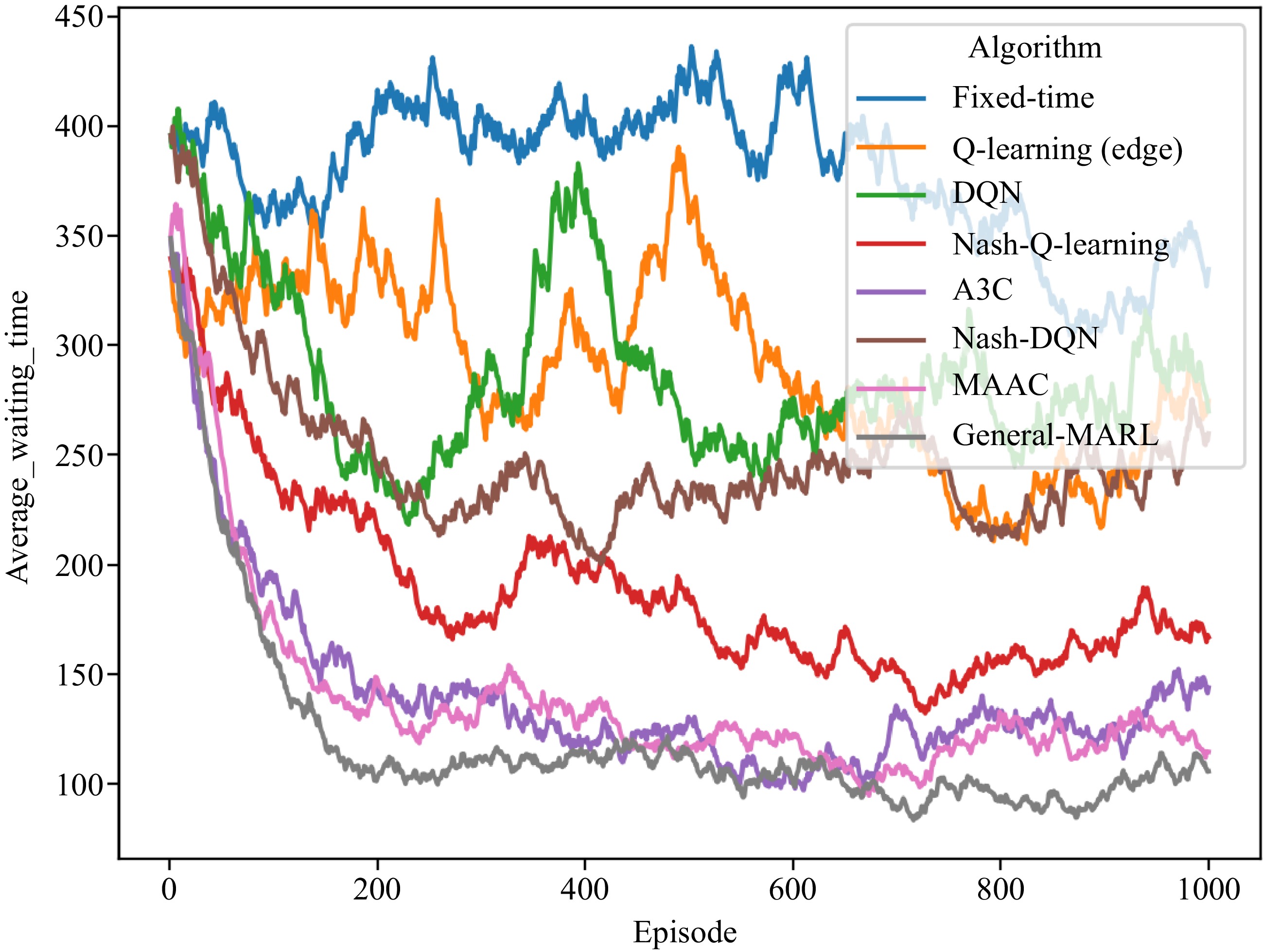
Figure 11. 

Multi-intersection traffic signal control training process (with network delay).

Experimental results

The results of the experiment are also split into two parts: the first part ignores network delay, and the second part considers network delay.

Ignoring network delay

After training in the simulation experiment in the previous section, 500 episode tests were performed to generate the experimental results, as shown in Table 2.

The experimental results show that, regarding the average speed and average waiting time of vehicles at 27 intersections, the General-MARL algorithm leads a similar performance as the Nash-DQN algorithm. The performance of General-MARL is not outstanding when network delay is ignored, but the overall performance of General-MARL is better than other baseline algorithms.

Considering network delay

We conduct 500 episodes in the tests after training in the simulation and collected the experimental results, as shown in Table 3. Regarding the average waiting time at intersections, the overall performance of General-MARL is the best, surpassing all the other algorithms, and it shows an average decrease of 18.3% waiting time compared to the baseline algorithms. As for the average speed of vehicles at intersections, the General-MARL algorithm increases the average speed by 10.2% when network delay is considered. As shown in Table 4, the General-MARL algorithm fully exceeds the baseline algorithms and other algorithms in terms of the accumulated waiting time of vehicles, network delay time, and delay rate indicators. The delay rate is reduced by 7.4%. Furthermore, the General- MARL algorithm optimizes each intersection to a certain extent, as shown in Table 5.

Overall analysis

The analysis of experimental results reveals that network delay has a significant impact on the actual application effect of the TSC algorithm. Although General-MARL showed good performance even when network delay was ignored, implementation of the method in urban TSC should take into account the influence of network latency for industrial deployment.

With the consideration of network delay, the General-MARL fully surpasses the baseline algorithms on average vehicle speed at intersection, average vehicle waiting time, vehicle cumulative waiting time, network delay time, and the indicators of delay rate. The average speed of vehicles increases by 23.2%, and the network latency decreases by 11.7%, as shown in Fig.12.

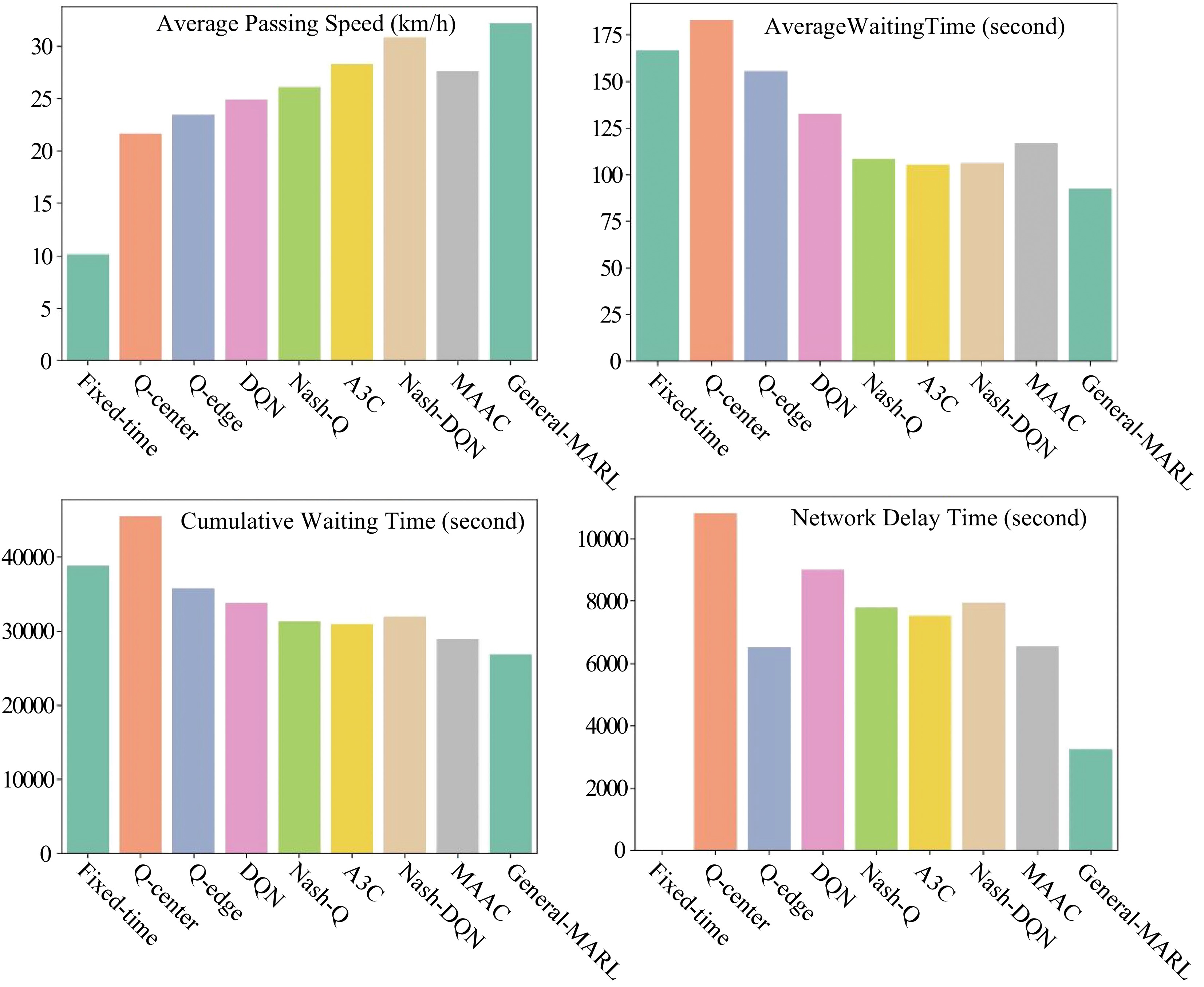
Figure 12. 

Comparative results among different algorithms.

In this paper, we proposed an integrated and cooperative IoT architecture GCTCS and the General-MARL algorithm for multi-intersection traffic signal control. The results from the proposed framework and algorithm showed that the average speed of vehicles was increased by 23.2%, and the network latency was reduced by 11.7%, when compared with baseline algorithms. Our results proved that the application of MARL in urban traffic signal control needs to consider multiple factors, including the simulation environment, algorithm process, deployment architecture, and network delay. The results also validated the best performance of the proposed General-MARL. Therefore, GCTCS and General-MARL showed great potential in practical applications and theoretical contributions for multi-intersection traffic signal control with large-scale deployment in real road networks.

In traffic signal control, not only the vehicles' but also the pedestrians' behaviours^[52], such as crossing times and waiting times are affected. In future studies, pedestrians will be included to cover all the road users at intersections. We will be able to further validate our proposed methodology based on real-life case studies because we have been invited by one city from China to deploy our GCTCS and algorithm in a test area.