A data-driven spatial-temporal model for prediction of tunnel deformation

As transportation infrastructure transitions from construction to operation and maintenance, the intelligent diagnosis of infrastructure structures has become a research focus. For tunnels, as operational time increases, it inevitably leads to structural deformation^[1,2]. Tunnels constructed under complex geological conditions present higher operational risks, making the long-term monitoring of deformation more urgent. Therefore, whether from the perspective of disease prevention or preventive maintenance, it is extremely necessary to carry out reasonable long-term performance monitoring and prediction of tunnel deformation.

Currently, the primary method for observation of tunnel deformation is structural health monitoring. Researchers have conducted extensive studies in sensor technology and monitoring systems. Wang et al. summarized the application of sensor technology in structural deformation monitoring during tunnel construction, discussing the advantages of different measuring devices and future directions^[3]. Barzegar et al. pointed out that utilizing wireless sensor network technology for monitoring tunnel convergence can reduce maintenance costs and the complexity of information transmission^[4]. Zhu et al. developed a real-time monitoring and warning system for tunnel deformation based on wireless sensor network technology, analyzing the deformation situation during tunnel excavation^[5]. Wang et al. utilized wireless inclinometer sensors to monitor the horizontal convergence of shield tunnels and validated the optimal installation positions through numerical simulations^[6]. Ding et al. employed a data fusion method using gyroscopes and strain gauges to predict tunnel deformation during the construction process^[7]. From the above studies, it is found that the monitoring of tunnel deformation mainly focuses on the construction period, with fewer studies on the operational phase. Additionally, tunnel deformation results from the combined effect of multiple factors^[8]. Thus, adopting multi-source sensors for monitoring tunnel structural performance during operation is necessary.

Recently, deformation prediction methods based on deep learning have been widely applied^[9,10]. Lai et al. developed a tunnel deformation model based on Artificial Neural Networks (ANN), and the results showed that it provided high accuracy in predicting soft soil tunnel deformations, making it a useful reference tool for practical engineering applications^[11]. He & Chen utilized a recursive neural network algorithm to model and analyze tunnel monitoring data, establishing a Long Short-Term Memory (LSTM) model to predict crown settlement^[12]. Cao et al. combined Empirical Mode Decomposition (EMD) with LSTM models, enhancing the accuracy of deformation prediction by increasing data dimensionality^[13]. However, the studies mentioned above only analyzed tunnel deformation from a temporal perspective, lacking consideration for deformation location.

Scholars have also conducted related research on deep learning methods that integrate both temporal and spatial dimensions. Tan et al. proposed a deep attention-temporal convolutional network method to predict the mechanical behavior of tunnel structures^[14]. Chen et al. constructed a tunnel settlement prediction dataset incorporating geological and construction parameters. They proposed a fusion network algorithm integrating spatial and temporal aspects for tunnel excavation^[15]. Maes et al.^[16] conducted long-term monitoring of strain, temperature, and deformation data in tunnels, and constructed a Principal Component Analysis (PCA) model to detect outliers based on the dependencies within the data. Zhou designed a Transformer-based model to analyze the ability of deep learning methods to handle the high-dimensional correlations between face deformation and nearby deformation data^[17]. However, the above methods have not been applied in tunnel deformation prediction and lack analysis of prediction accuracy at different locations.

Based on the above problems, this paper proposes a data-driven spatial-temporal approach to predict deformation, considering stress, strain, temperature, and deformation during the operational phase of tunnels. The coupled network integrates Graph Attention Networks (GAT) and Gated Recurrent Unit (GRU) algorithms. It captures multi-source sensor information at different spatial nodes and learns temporal dependencies to predict tunnel deformation at various nodes. Additionally, experiments were conducted to validate the predictive capabilities of the model. This study introduces a novel deformation prediction method, and the findings can also facilitate the application of deep learning algorithms in other transportation infrastructures.

In this section, a spatial-temporal coupled network model is proposed for real-time prediction of tunnel deformation behavior. Firstly, an adjacency matrix is constructed based on the spatial relationships between monitoring locations in the tunnel. Then, the GAT algorithm is employed to extract features between different nodes. Subsequently, the features of each node are used as inputs for each GRU algorithm. The deformation of each node in the future is predicted through model training. The framework of this method is illustrated in Fig. 1.

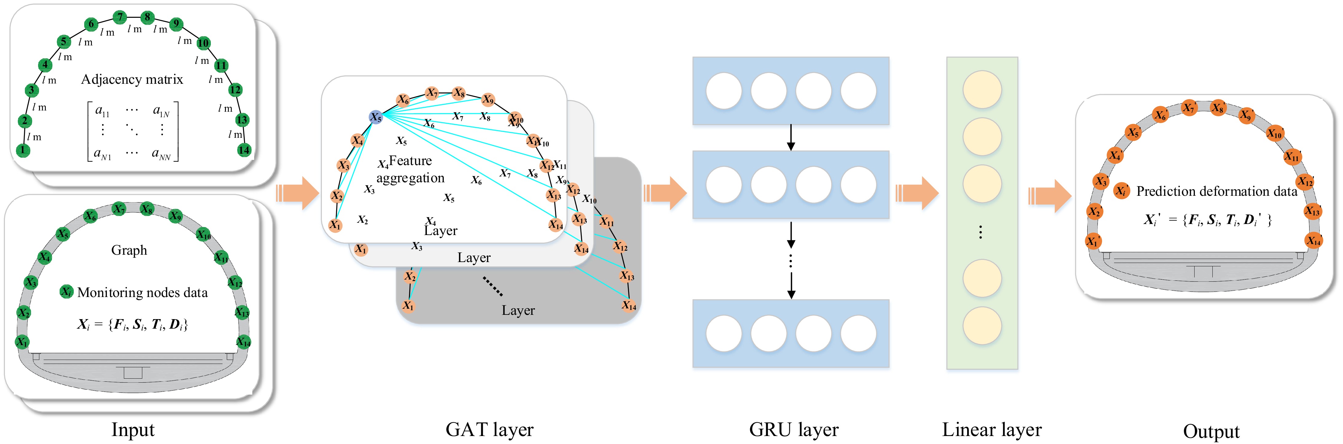
Figure 1. 

The framework of the deformation prediction method.

Parameter definitions

The cross-section of a tunnel can be viewed as a natural graph structure. Each monitoring position can be considered a spatial node in the cross-section. Therefore, studying the relationships between different monitoring positions in the tunnel cross-section is meaningful research. To explore the influence of different factors on deformation, stress, strain, temperature, and displacement sensors are installed at each node. Supposing there are N nodes in the cross-section, the data at node i can be defined as X_i = {F_i, S_i, T_i, D_i}, where $ i \in \left[ {1,N} \right] $.

Each sensor's collected data can be regarded as a time series, and studying the evolution pattern of monitoring data over time is also essential. If the monitoring data of all nodes is defined as X, the data at time t can be represented as $ {{\boldsymbol{X}}^t} = \left\{ {{\boldsymbol{X}}_1^t,{\boldsymbol{X}}_2^t, \cdots ,{\boldsymbol{X}}_N^t} \right\} $. Assuming the total monitoring period is H, the data matrix can be represented as $ {\boldsymbol{X}} \in {R^{H \times N \times 4}} $.

If p is defined as the input time length, the model will utilize data from the past p time steps to predict deformation data for the future time step. At time t, this process can be represented as:

where, $ {{\boldsymbol{X}}^{t - p + 1:t}} $ is the data in the past p steps; F(X) is the prediction method; $ {{\boldsymbol{X'}}^{t + 1}} $ is the prediction result of in next moment, $ {\boldsymbol{X'}}_i^{t + 1} = \{ {\boldsymbol{F}}_i^{t + 1},{\boldsymbol{S}}_i^{t + 1},{\boldsymbol{T}}_i^{t + 1},{\boldsymbol{D'}}_N^{t + 1}\} $.

Spatial feature extraction

Due to the continuous nature of tunnel section structures, the generation of deformation requires consideration of the mutual influence between nodes. This paper constructs a spatial graph G^t = (X^t, E), using the distance relationships between different nodes E as edges, to represent the structural monitoring data graph at time t. When the distance between nodes is greater, the degree of mutual influence between them is smaller. Therefore, the adjacency matrix can be approximated as:

where, a_ij represents the weight between node i and j; n_i and n_j are the spatial positions of nodes i and j.

The GAT algorithm is employed to learn the weights between nodes, enabling the model to dynamically focus on important neighboring nodes to better capture the complex relationships between nodes. For the node X_i and its neighbor C(X_i), the node feature updating method is represented as:

where, $ v_{{{\boldsymbol{X}}_i}}^{(l)} $ is the representation of a node X_i in the l-th layer; $ \sigma $ is the activation function; $ \alpha _{{{\boldsymbol{X}}_i}{{\boldsymbol{X}}_j}}^{(l)} $ is the attention coefficient between the node X_i and its neighbor X_j.

Temporal feature extraction

The GRU layer is added to the model to capture the temporal dependencies between different nodes. In this model, monitoring data is first passed to the GAT layer for spatial feature extraction, and then transferred to the GRU layer for time feature learning. The process is illustrated in Fig. 2.

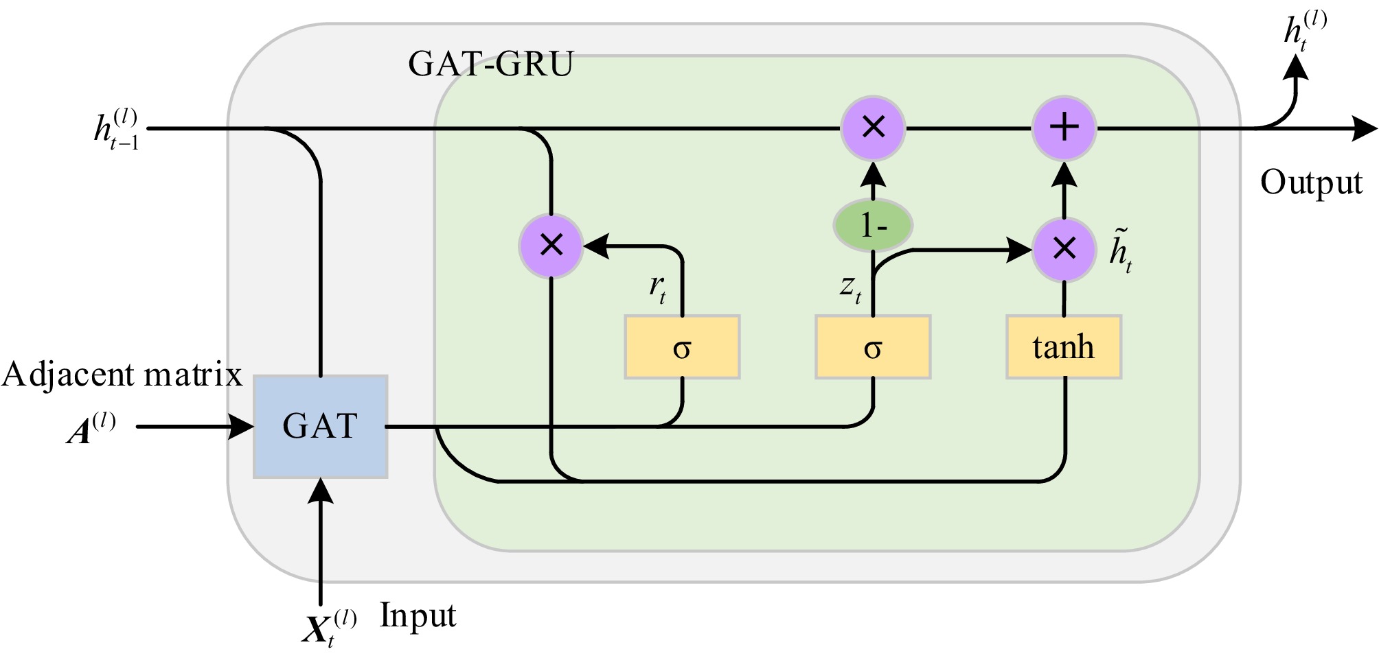
Figure 2. 

Structure of the GAT-GRU network.

At each time step t, the output $ v_{{{\boldsymbol{X}}_i}}^{(l)} $ of the GAT layer will serve as the input $ h_t^{(l)} $ to the GRU. According to the hidden state $ h_{t - 1}^{(l)} $ of the previous time step, the update process is formulated as Eqns (5)−(8).

where, r_t, z_t, and $ {\tilde h_t} $ respectively represent the reset gate, update gate, and candidate update. W_r, W_z, and W_h are the weight parameters; b_r, b_z, and b_h are the biases; σ and tanh are activation functions.

To validate the accuracy of the proposed model, a tunnel located in Shandong Province, China, was selected as a typical case study. The tunnel achieved full completion in January 2024 and is a newly constructed tunnel. However, it traverses challenging terrain with frequent changes in rock mass quality and is also an exceptionally long tunnel. It is necessary to conduct real-time deformation monitoring. The deformation monitoring system was installed on the right side of the tunnel, with monitoring nodes set up every 2 m. The positions and layout of the deformation monitoring system are illustrated in Fig. 3.

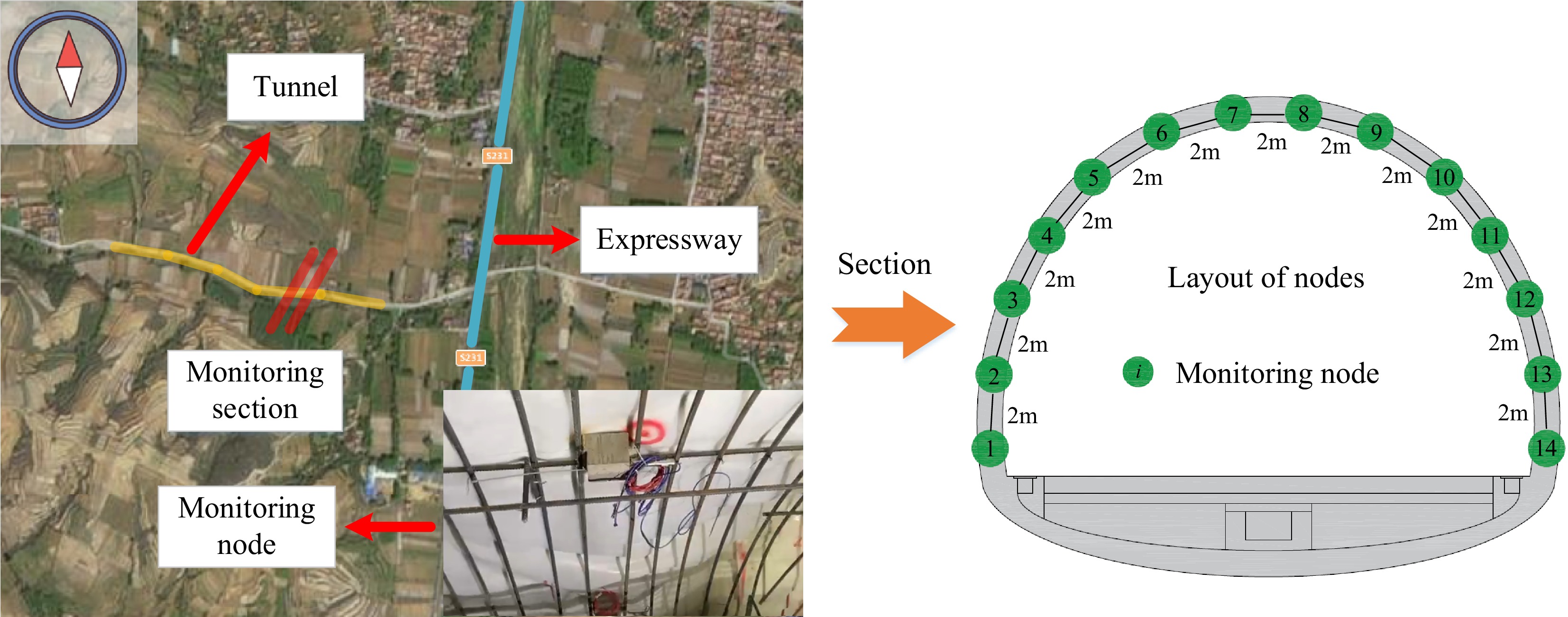
Figure 3. 

Location and layout of the deformation monitoring system.

The data collection frequency is once per hour, with each monitoring node containing four types of data: stress, strain, temperature, and displacement. Figure 4 shows the monitoring data at node 7, located at the crown of the tunnel. Since the sensors were installed during the initial lining stage of the construction period, the initial monitoring values obtained at the start of the monitoring system's operation are used as the baseline values for data analysis. The data illustrated fluctuations from the first day of tunnel operation until the end of March. It can be observed that the data for each factor exhibited periodic variations and showed significant correlations. Specifically, stress and temperature were negatively correlated with deformation, while strain was positively correlated with deformation.

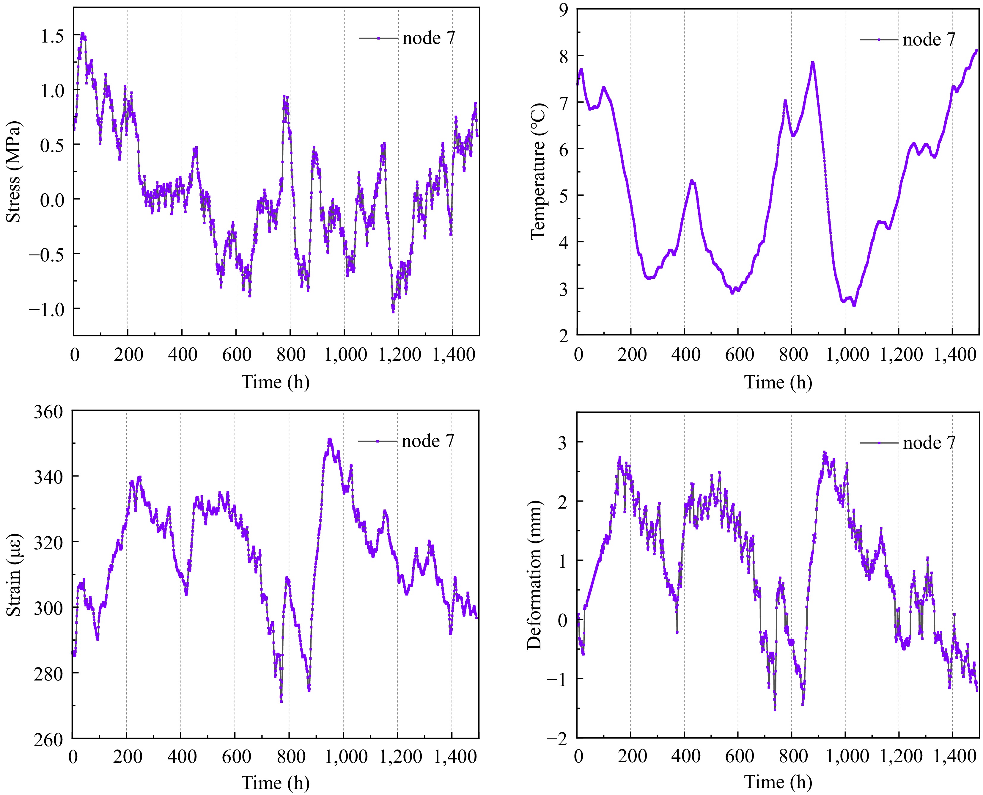
Figure 4. 

Monitoring data of different factors. (a) Stress, (b) temperature, (c) strain, and (d) deformation.

Prediction results and discussion

Firstly, according to the dataset format defined in this paper's parameter definition, the monitoring data was organized into the $ {\boldsymbol{X}} \in {R^{H \times N \times 4}} $. Secondly, each node's data was normalized to eliminate differences in data magnitudes between different factors. The normalization formula is shown as Eqn (9).

where, j represents the different factors, $ j \in [1,4] $.

This paper uses two metrics, Mean Absolute Error (MAE) and Root Mean Square Error (RMSE), to evaluate the accuracy of the proposed prediction model. The formulas for different metrics are as follows:

where, $ {{\boldsymbol{D'_{:,i,k}}}} $ and $ {{\boldsymbol{D}}_{:,i,k}} $ respectively represent the predicted value and actual value of the k-th deformation data for the i-th monitoring node.

The data used in this study was collected from January 16, 2024, to March 18, 2024. The data collection interval is 1 h, providing hourly data on various factors including stress, strain, temperature, and deformation at multiple monitoring points along the cross-section. The preprocessed data was divided into training and testing sets at a ratio of 7:3. Since different model hyperparameters could affect the model's performance, this paper employed grid search to explore parameter combinations and selected the optimal predictive performance as the combination scheme. Grid search generates all possible combinations of hyperparameter values within their specified ranges, then trains and evaluates the model for each combination, ultimately selecting the combination with the best performance. The parameter selection ranges and optimal parameters are presented in Table 1.

To validate the modeling capability of the GAT-GRU model, a comparative analysis was conducted on the prediction results of other models. A total of two temporal prediction models, three spatial prediction models, and their best-performing combinations were selected. These include GRU, Temporal Convolutional Network (TCN), Chebyshev Network (ChebNet), Graph Convolutional Network (GCN), GAT, GAT-TCN, and GAT-GRU. Table 2 shows the average predictive capabilities of different models for all monitoring positions. When MAE and RMSE are smaller, it indicates that the model has better predictive performance.

The comparison of different models reveals that the coupled GAT-GRU model demonstrates the best-fitting performance in testing. Its MAE and RMSE are 0.042 and 0.059 mm, respectively, representing an improvement in accuracy of 43.2% and 40.4%, compared to the GAT-TCN model. Furthermore, single temporal or spatial prediction models struggle to predict tunnel deformation effectively. In terms of temporal prediction models, the GRU model exhibits stronger temporal dependency than the TCN, resulting in higher prediction accuracy. As for spatial prediction models, the GAT model outperforms the GCN and ChebNet models, with a decrease in MAE of over 0.1 mm and a decrease in RMSE of over 0.2 mm.

Figure 5 summarizes the accuracy of each model at the tunnel's different locations. It is found that at certain monitoring nodes, the predictive performance is significantly lower than the average level, indicating the presence of underfitting issues. Except for the GAT-TCN and GAT-GRU models, the interquartile range (IQR) of the remaining models is around 0.8 mm. This indicates significant variability in predictive capability among different nodes, and these models cannot predict tunnel deformations well at various locations. Among all models, the GAT-GRU model demonstrates the best fit to the normal curve, with all statistical metrics being optimal. The MAE and RMSE for each node are both less than 0.1 mm.

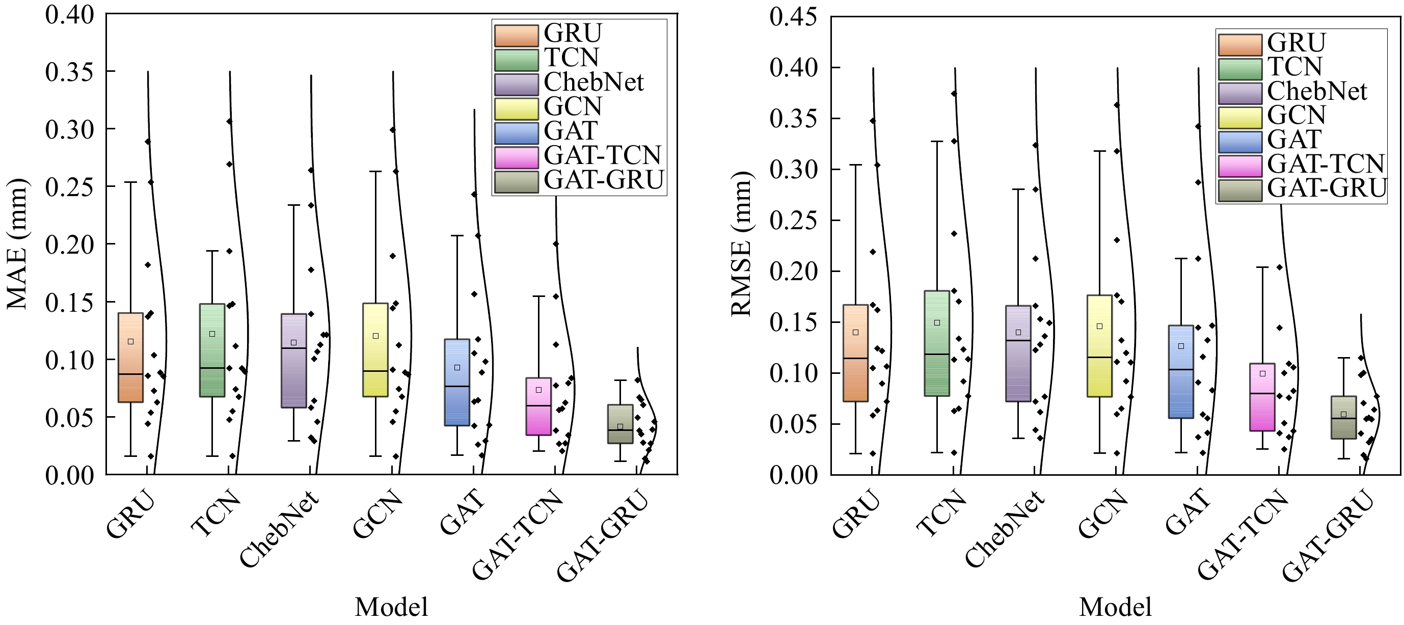
Figure 5. 

Comparison of the accuracy of different models at different monitoring locations. (a) MAE, and (b) RMSE.

The distribution of MAE values for each node is shown in Fig. 6a. From the side to the crown of the tunnel, the prediction accuracy gradually increases. Among them, the model predictions are best at the crown, with MAE values for nodes 5 to 10 all below 0.1 mm. The errors are largest at the side, with the accuracy at the left side of the tunnel significantly lower than the right side. At node 1, its MAE error reaches 0.3 mm. The prediction accuracy for the side nodes (e.g., nodes 1 and 14) is less satisfactory compared to the crown node (e.g., node 7). This can be attributed to the structural and mechanical characteristics of the tunnel. The crown is centrally located and experiences relatively uniform stress distribution and stable deformation, resulting in higher prediction accuracy. In contrast, the side nodes are subjected to more complex stress conditions, including horizontal and vertical stress components, and exhibit greater variability in deformation due to their proximity to the tunnel boundaries and interaction with the surrounding rock. These factors increase the difficulty of accurately modeling deformation patterns. Additionally, geological heterogeneities and potential variations in support quality along the sides may further contribute to the reduced prediction performance for these nodes.

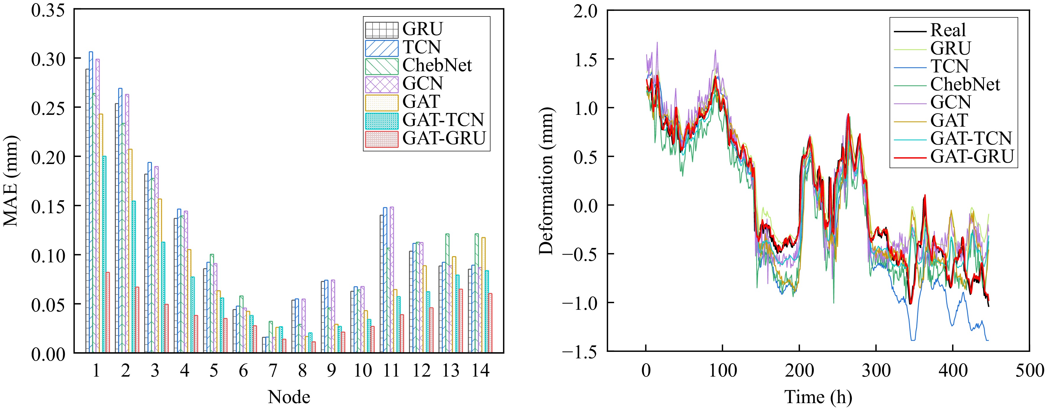
Figure 6. 

Comparison of prediction results for each model. (a) MAE at each node, (b) typical node (node 1).

To further analyze the underfitting situation, Fig. 6b presents the prediction results of each model at node 1. In the early stages of prediction, all models fit well. However, over time, except for the GAT-GRU model, other methods experience model drift, resulting in a deterioration in prediction performance.

To further test the predictive capability of the model, this study conducted a sensitivity analysis. The stability of the model was discussed about two parameters: the length of the time step and the prediction scale. It is important to note that the model's time granularity was set to the minimum granularity of 1 h.

First, the influence of the time step on accuracy was investigated. Setting the prediction time to 1 h and keeping other parameters as selected values in Table 1, the predictive performance of the model was tested for time steps ranging from 3 to 15 h. As shown in Fig. 7a, the model's accuracy exhibits periodic fluctuations. When the prediction time is 10 h, the model's error is the highest, with MAE and RMSE values of 0.096 and 0.135 mm, respectively. When the prediction time is 6 and 7 h, the model's predictive accuracy is the highest, with RMSE values of 0.059 mm each. This suggests that historical data from the past 6 to 7 h is crucial for analyzing future tunnel deformations.

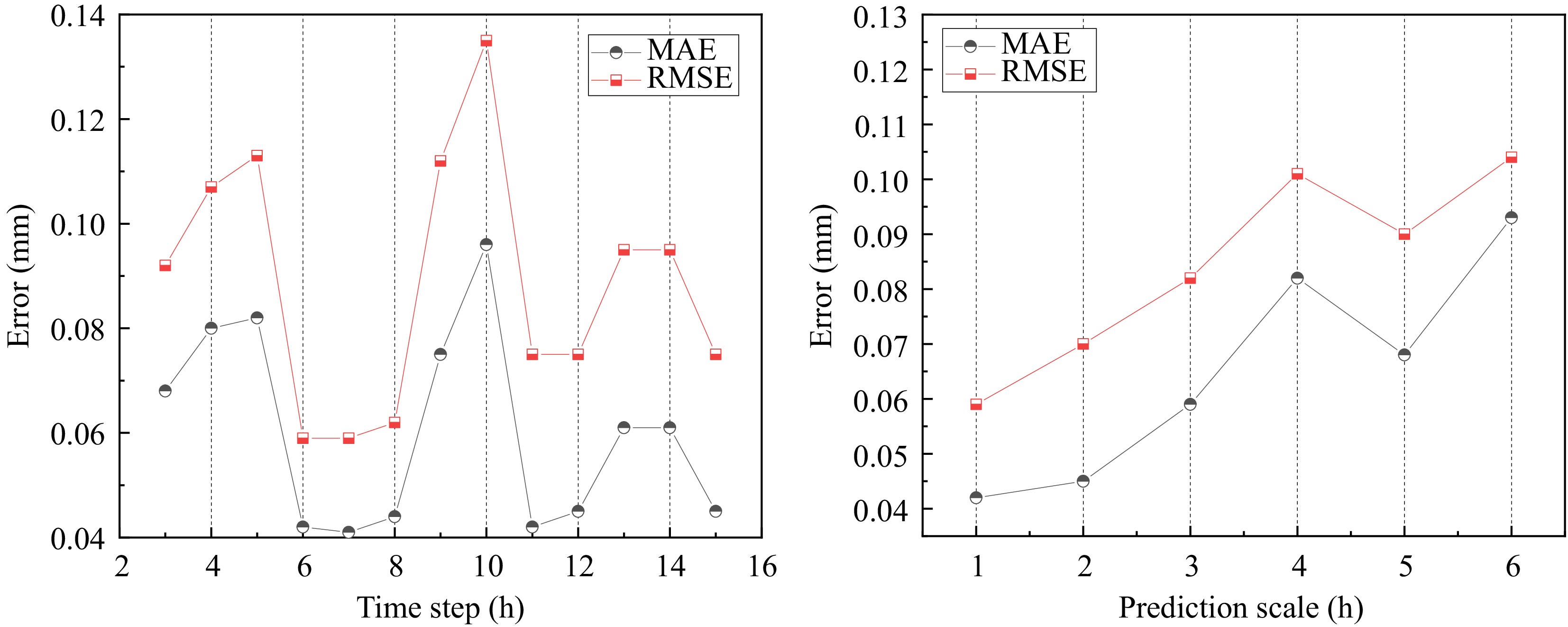
Figure 7. 

The predictive capability of the model under different conditions. (a) Time step, and (b) prediction scale.

Afterward, the impact of different prediction scales on the fitting effect was discussed. Setting the time step to 6 h, the model error was analyzed for prediction scales ranging from 1 to 6 h, as shown in Fig. 7b. The results indicate that with the increase of the prediction scale, the error shows an overall increasing trend. When the prediction time is within 5 h, both MAE and RMSE of the model are less than 0.1 mm. This suggests that the predictive performance of the model decreases with increasing time, but within the next 5 h, it is still able to predict tunnel deformations relatively well.

This paper proposed a spatial-temporal coupled deep learning model for real-time prediction of tunnel deformation behavior. The model considered multiple variables including stress, strain, temperature, and deformation, enhancing the practical engineering credibility of the prediction results. The main conclusions are as follows:

(1) The proposed model exhibits formidable predictive capability. A comparison of a series of spatial and temporal prediction models was conducted. The results indicated that single models faced challenges in effectively predicting tunnel deformations. Additionally, the GAT-GRU framework proposed in this paper exhibited optimal fitting performance. The model achieved an MAE of 0.042 mm and an RMSE of 0.059 mm, respectively.

(2) The predictive performance at different monitoring locations was analyzed. The results indicated that the fitting accuracy is highest at the tunnel crown, with the MAE of all models being less than 0.1 mm. However, there were larger prediction errors at the tunnel side, suggesting that the side is subject to more interference, resulting in greater data fluctuations that affect the performance of the models.

(3) The robustness of the model was analyzed under different time steps and prediction scales. The experiments showed that the past 6−7 h had the greatest impact on future tunnel deformation. As the prediction scale increased, the accuracy gradually decreased, but still could effectively predict the deformation within the future 5 h.