Nitrogen response and growth trajectory of sorghum CRISPR-Cas9 mutants using high-throughput phenotyping

Modern agriculture has become increasingly mechanized and specialized, heavily dependent on fossil fuels as the main energy source and on the application of large amounts of chemical fertilizers to improve productivity. Since the invention of the Haber–Bosch process, nitrogen (N) fertilizer has been increasingly used in crop production, leading to 30%–50% of crop yield gain^[1,2]. Global data for the use of N fertilizer for the three major cereal crops (maize, rice, and wheat) indicate that only 18%–49% of the applied N is taken up by these crops, with the remainder being lost to runoff, leaching into waterways, and volatilization^[3,4]. The excessive application of inorganic N fertilizer has adverse effects on biodiversity and poses threats to human and animal health within the agroecosystem^[4]. The increasing demand for sustainable agriculture provides new challenges for plant breeding and genetics, where achieving comparable yields while maintaining soil and environmental health requires reducing chemical fertilizer inputs and minimizing carbon footprints^[5]. In addition, CRISPR-Cas9-based gene editing has provided unprecedented efficiency in mutant genesis. Therefore, it is critical to investigate the genes responsible for crop N responses via reverse genetics to inform future plant breeding practices.

Sorghum is the fifth most grown cereal crop globally, with approximately half a billion people, mainly in developing countries, relying on it for food security^[6]. In contrast to recently developed maize hybrids optimized for high N cultivation to enhance economic productivity, such as in the U.S. Corn Belt^[7,8], Sorghum cultivars exhibit significant diversity in N use efficiency (NUE), stemming from their natural adaptation in varied fertility environments^[9]. The NUE diversity positions sorghum as an ideal model C4 crop for investigating plant responses to N deficiency and NUE in crop production. N deficiency has been reported to systematically impact various aspects of sorghum growth, spanning from morphological traits, such as leaf area, tiller number, and plant height, to developmental characteristics, like flowering time and leaf senescence, as well as physiological traits, including chlorophyll content, protein content, plant hormone metabolism, and membrane transport, among others^[10−13]. These changes in phenotypes ultimately reflect the interactions between the plant genetics and its low N environment, leading to decreased photosynthesis efficiency and reduced biomass production^[14,15].

CRISPR-Cas9-based gene editing has emerged as a revolutionary tool for introducing genetic variation into plant cells, enabling a wide range of applications including gene knockouts, base editing, prime editing, homology-directed repair, targeted gene activation or silencing, and epigenomic editing^[16,17]. Compared to conventional mutagenesis approaches, such as EMS or T-DNA insertion, CRISPR-Cas9 enables the precise generation of mutants in targeted genes, such as N-responsive genes, and therefore holds great potential for elucidating the molecular mechanisms underlying N responses in sorghum. Traditionally, researchers have used laboratory biochemistry methods to quantify phenotypic responses to N treatments to measure plant N and chlorophyll content and manually collected plant morphological traits^[10]. These methods are relatively cost- and labor-intensive, which often limits the sample density and sample size. High-throughput phenotyping is a set of phenotyping techniques, primarily focused on automated data acquisition at a large scale, that has recently emerged as an enabling tool for crop breeding and plant science research. Numerous high-throughput phenotyping studies have employed spectral or imaging techniques using sensors or cameras. These techniques have captured information ranging from red-green-blue (RGB) color to infrared, thermal, multispectral, and hyperspectral data^[18−23]. Previous studies have shown that plant structural phenotypes obtained from high-throughput phenotyping experiments, such as plant height, convex hull area, and pixel count, can be used as indicators of N levels in plants^[24,25].

Using a camera-based high-throughput phenotyping system coupled with automation, massive amounts of imagery data can be obtained daily, presenting new challenges for image data analysis and result interpretation. High-throughput phenotyping captures information about plants and their environment with inherent noise. Domain knowledge in plant biology and appropriate experimental design are essential for developing models that distinguish noise from informative variables, which may mediate, covary with, or interact with the features of interest. Additionally, high-throughput phenotyping enables non-destructive measurements across crop growth stages and often generates high-dimensional temporal data. An intuitive and widely applicable approach is to treat each time point as a phenotype. Comparisons between the factors of interest can be made directly for each time point by statistical models such as ANOVA, after which the biological significance is summarized^[26,27]. To gain deeper insight into the mechanisms underlying crop development, functional analysis of variance (FANOVA) was employed to decompose the temporal variance into factors such as genotype and treatment^[28,29]. Functional principal component (FPC) analysis, a functional-based factor model, has been shown to associate FPCs representing growth trajectory characteristics with genomic markers or QTLs^[30,31]. Recently, researchers have used latent space phenotyping methods to automatically learn hidden parameters that represent the response to treatment and are associated with the genomic data^[32−34]. These approaches captured overall visually evident features from plant imagery data or spectra data without the need to construct and extract features using conventional modeling methods. However, the interpretation of such latent space phenotypes can be challenging.

In our previous study^[35], a comparative transcriptome analysis was performed to investigate nitrogen response across various plants. Specifically, sorghum's response to varying nutrient availability (ammonium, nitrate, and urea) was examined by analyzing both differential gene expression and co-expression patterns. A nitrogen-responsive co-expression module in root tissue was identified, centered around two hub genes: Sobic.001G040200 (encoding a NAC transcription factor) and Sobic.002G121300 (encoding a serine carboxypeptidase). Further analysis of the immediate network of these hub genes focused on their direct nodes to assess their potential roles in nitrogen metabolism and assimilation. This investigation led to the identification of 12 genes within the module with putative nitrogen-related functions. In the current study, an in-depth characterization of six of these 12 genes was worked on (Supplementary Table S1, S2 & Supplementary Fig. S1). Leveraging the in-house generated CRISPR-Cas9 mutants in sorghum, the study presents a pipeline for characterizing plant growth responses to different N treatments. The pipeline utilizes the automated plant imaging system, combining it with computer vision methods to extract phenotypes and statistical modeling to summarize the high-dimensional temporal phenotype into biologically meaningful parameters. This data acquisition and analytical pipeline paves the way for a better understanding of N responses in CRISPR-Cas9 edited mutants, shedding light on facilitating plant breeding.

The study utilized the CRISPR-Cas9 technique to edit the candidate genes selected from a previous study^[35]. After selecting the successful edit events and selfing for four generations, five different edited lines were obtained (named Edit1 to Edit5, see Supplementary Table S1), with one to three homozygous knocked-out candidate genes in each genotype. The five gene-edited sorghum lines and the Tx430 control were planted in small pots at the Greenhouse Innovation Center of the University of Nebraska-Lincoln on March 23, 2022. Healthily germinated plants were transferred to 1.5-gallon pots on April 14, 2022. Each 1.5-gallon pot contained soil composed of two-thirds peat moss, one-third vermiculite, and 1.5 kilograms of lime per cubic meter of soil, which contained no N fertilizer. From planting to April 21, 2022, 20-10-20 N-phosphorus-potassium liquid fertilizer was applied to saturation to ensure the seedlings' survival.

The plants were placed on the belts of the LemnaTec3D automated imaging system (LemnaTec GmbH, Aachen, Germany) following a randomized complete block design, which contained three blocks and each block consisted of 12 plants, a full replication of six genotypes grown in 2 N conditions. 53.6 g N-free Hoagland medium powder (bioWORLD Molecular Life Sciences, USA) and potassium nitrate (60.66 g for high N or 12.13 g for low N) were diluted to 40 L with fertilizer-free water in the greenhouse to make 15 mM N or 3 mM N nutrient solutions. The solutions were applied to 250 mL of each pot twice a week. The same solutions were prepared every two weeks and stored in the dark room to avoid the growth of algae. Additional water was applied to each pot every day. In total, 36 plants were imaged. The imaging started on April 21, 2022, and terminated on August 4, 2022.

Dry weight measurement

The whole plants from the experiment on August 4^th, 2022, for 130 DAS were harvested. The roots were carefully shaken and washed, after which the plants were dried in a 65 °C dryer for 5 d. Then the dry weight of the plant was measured separately for the shoot, root, and panicle.

Image segmentation

To segment the plant pixels from the background, a customized Python script with multiple computer vision functions imported from OpenCV 4.1.0.25 was used^[36]. More specifically, a binary mask was constructed for the plant by subtracting the pixel values of a background-only image from every plant image, followed by Otsu binarization^[37] of the green channel. Ideally, only the plant area has non-zero pixels in the resulting binary mask, but some noise may exist. To denoise, the mask and the image were cropped along all four edges to remove residues from the frame of the imaging chamber and the pot, due to the imperfection of the overlap between the plant image and the background image. Image opening and closing morphological operations were applied with a 5-by-5 square structure element to remove the salt and pepper noise. Finally, the binary mask was multiplied with the raw image to obtain the segmented image.

Phenotypic traits extraction from imagery data

The segmented images were used to extract plant phenotypic traits, including pixel-coordinates-based traits such as plant height, plant width, and pixel coverage, and color-based vegetation indices. The plant pixel coverage was measured as the total number of non-zero pixels in a segmented image. This number is comparable across the images since all the images are of the same dimension. The plant height was measured from the vertical axis value of the first non-zero pixel from the bottom to the first non-zero pixel from the top. The plant width was measured from the horizontal axis value of the first non-zero pixel from the left to the first non-zero pixel from the right. The formulas for the calculation of vegetation indices were as shown by Rodene et al.^[27]. Briefly, the values of the RGB channels were used, and average values across all the segmented pixels were recorded.

Statistical modeling of growth dynamics

The following logistic function was used to model the growth dynamics of the pixel count of sorghum. The pixel count on the x^th day after sowing is modeled as:

where, A was the carrying capacity, µ was the inflection point, and k was the steepness. The first derivative of the pixel count:

was used to calculate the slope at the inflection point f(µ) = Ak/4, which represented the maximum growth rate.

A Gaussian peak function was used to model the sorghum ExG index growth dynamics. The ExG on the x^th day after sowing was modeled as:

where, a was the amplitude, b was the critical point, c was the width parameter, and d was the vertical adjustment of the curve. The maximum ExG, which was reached when DAS equaled b, was controlled by both the amplitude and the vertical adjustment. Therefore, it was calculated as a + d. In addition, the c parameter described the width of the peak, which was considered as a measurement of the stay-green phenotype. It corresponds to the distance between the DAS of the peak and the inflection point, which shows the highest or lowest slope, at either side.

All parameters were solved for each of the 36 plants using nonlinear least squares regression as implemented in Scipy v1.12.0^[38]. The parameters and derived traits were analyzed using analysis of variance (ANOVA). The differences of high N and low N within each genotype were compared using F-contrasts.

Previous transcriptomic analysis^[35] identified a series of N-responsiveness hub genes. In the current study, using CRISPRCas9 technology^[39], five gene-edited sorghum lines in the Tx430 background were obtained, with up to three genes from the previous study being knocked out for each homozygous mutant (see Supplementary Table S1 & S2). These gene-edited sorghum mutants and Tx430 wildtype (WT) were grown at the LemnaTec high-throughput plant phenotyping platform with two different N treatments: high N (15 mM nitrate) and low N (3 mM nitrate)^[40]. The experiment was conducted following a complete randomized block design with three replications per genotype (Fig. 1a, Materials and Methods).

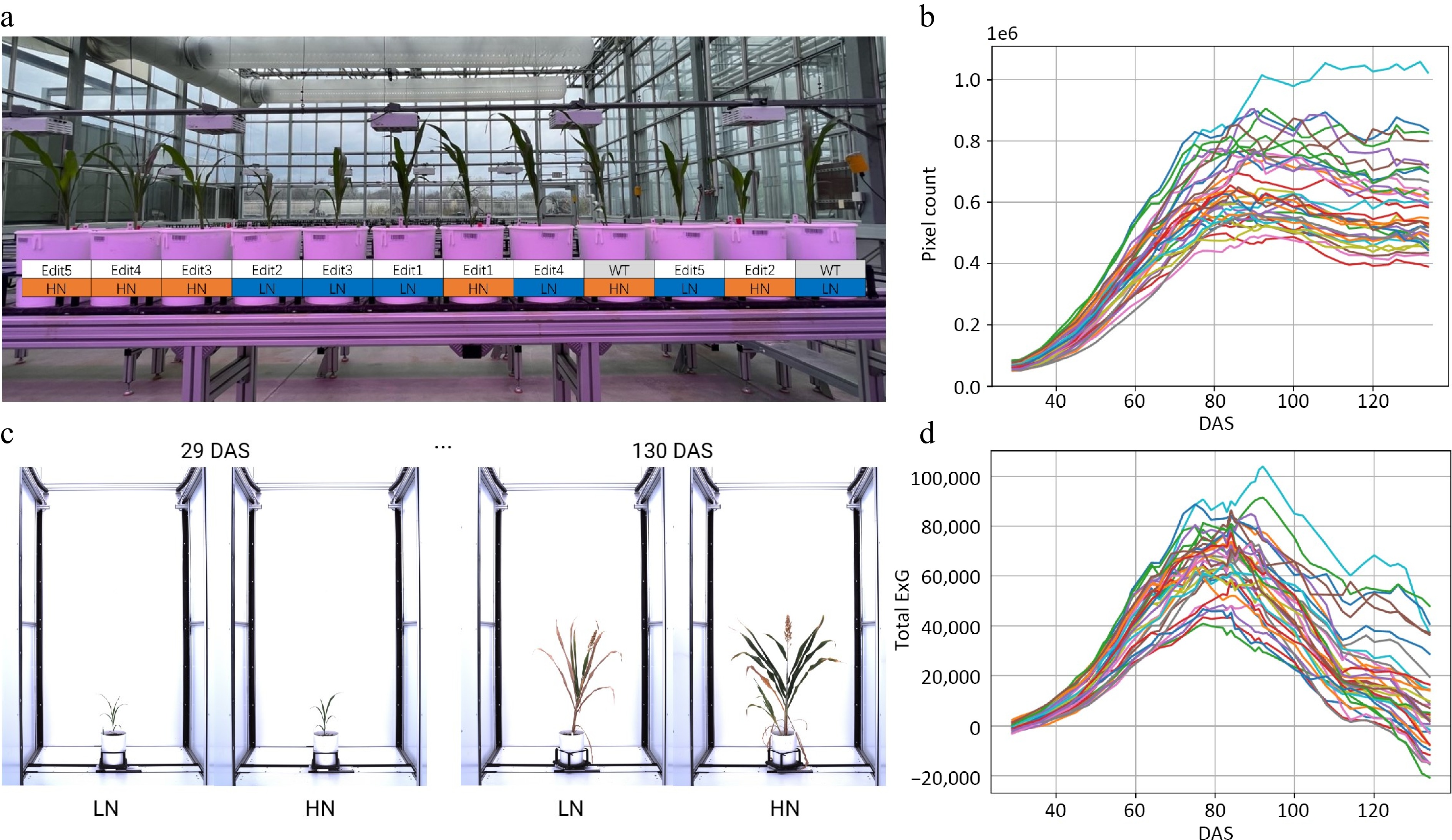
Figure 1. 

Characterizing sorghum CRISPR mutants for N responses using a high-throughput phenotyping procedure. (a) The greenhouse experimental design for CRISPR mutants under high N (15 mM) and low N (3 mM) conditions. (b) Time-series automatic image acquisition from the first day of phenotyping (29 DAS) to the last day of phenotyping (130 DAS). The examples are Tx430 WT. The extracted phenotypes. (c) Pixel count. (d) Total ExG index value for each individual during the phenotyping period.

Conventional phenotyping was also performed to assess the dry weight of the plant at the end point of the experiment. The Tx430 WT showed significantly increased dry weight accumulation under high N conditions in each part of the plant we measured, indicating its sensitivity and response to N treatment. The same trend was found for Edit4 and Edit5. Edit1, however, exhibited no significant difference in any of the dry weights between the two N treatments (Supplementary Fig. S2). Edit2 and Edit3 had similar phenotypes, in that the dry weight of the whole plant showed significant N responses (F test, p-values < 0.050), but this response was not observed in the dry weight measurement of separated root, shoot, or panicle. These results of conventional phenotyping suggested that N treatments significantly influenced sorghum growth, with distinct responses observed between various gene-edited lines. Tracking N responses in specific growth stages could reveal important details about how the N response has changed in these gene-edited lines.

For the high-throughput phenotyping, in total, 15,120 imagery data points were obtained in a time series manner at 42 different time points (Fig. 1b). A manually created background image was applied for background subtraction, followed by image opening and closing morphological operations to remove the potential 'salt and pepper noise' that remained in the background^[41]. This ensured more successful segmentation across different growth stages (Supplementary Fig. S3, see Materials and Methods), compared to color thresholding, where green tissues, panicles, and senescent tissues require different thresholds. Two phenotypic traits associated with plant growth and N content were extracted in a time-series manner, from which growth trajectories were then modeled and explained (Fig. 1c, d; Supplementary Tables S3 & S4).

Characterization of biomass growth trajectories using pixel count

The plant pixel count has been previously reported to be strongly correlated with fresh weight, which serves as a proxy for biomass^[42]. To study biomass dynamics using time-series imagery data, pixel counts for each plant on each imaging date were extracted from the segmented images and averaged for 10 different angles of side-view images. The plant pixel counts in our experiment followed an S-shaped curve (Fig. 2a), which can be fitted as a logistic function, consistent with a number of previous studies^[31,43]. The steepness, inflection point, and amplitude parameters (k, µ, and A) were estimated from the logistic growth curve by fitting the model (see Materials and Methods and Fig. 2a).

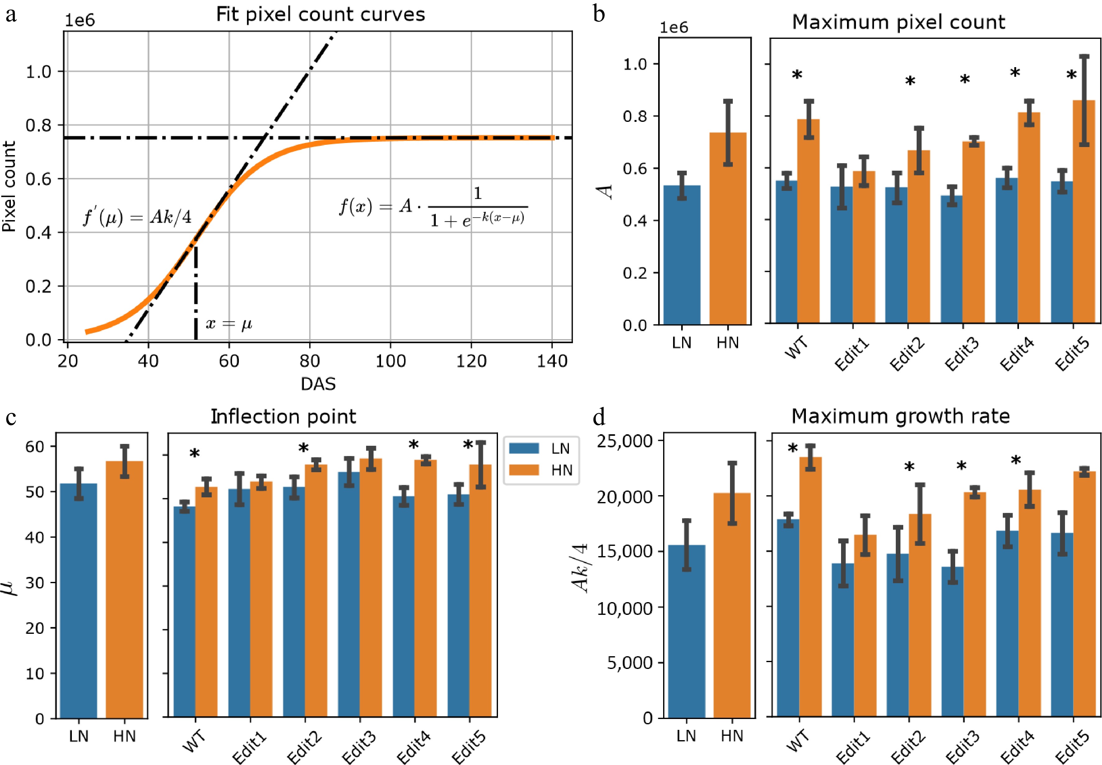
Figure 2. 

Modeling of the pixel count trait. (a) Logistic curves with the parameters estimated from the data. The bold lines represent the curves of WT Tx430 plants, and the dashed color lines represent the gene-edited lines. (b)−(d) The phenotypes estimated or derived from the function. The left panel shows the overall comparisons between treatment and the right panel shows the comparisons for each genotype. The error bars indicate the standard deviation. Stars indicate a significant difference between low N and high N treatment for the pooled data or within a single genotype.

After extracting estimated parameters, the results suggested that the maximum pixel counts (A), serving as a proxy for total biomass, exhibited a significant (ANOVA, p-value < 0.050) genotype effect and treatment effect (Supplementary Fig. S4 & Supplementary Table S5). When compared with the low N treatment group, overall significantly (F-test, p-value < 0.001) higher maximum pixel counts under high N condition were observed (Fig. 2b & Supplementary Table S5). Particularly, Tx430 WT and Edit3-5 showed significantly (F-test, p-value < 0.050, Supplementary Table S5) higher biomass (or A value) in high N than low N, but the trend was not found in Edit1 and Edit2. This observation is highly correlated with the dry weight measurements (Supplementary Fig. S2).

The parameter µ, representing the DAS when the fastest pixel count growth rate was achieved, may indicate the transition from vegetative growth, such as leaves and stalks, visually apparent from the images, to reproductive growth. The results suggested that overall, the plants achieved the fastest growth rate under high N than low N conditions (F-test, p-value < 0.001, Fig. 2c & Supplementary Table S3). Again, this pattern was not observed for Edit1 (F-test, p-value = 0.312, Supplementary Table S5). Consistently, the fastest growth rate, measured using Ak/4 (see Materials and Methods), indicated that there was an overall significantly faster rate (F-test, p-value < 0.050, Fig. 2d & Supplementary Table S5) when N was sufficient. Taken together, the data suggested that WT and Edit2-5 grew longer and faster, which was consistent with the hand-measured data that they accumulated more biomass under high N compared to low N conditions, while Edit1 appeared unresponsive to high N treatments.

Characterization of phenotypic dynamics using Excess Green indices

Next, a different trait—Excess Green (ExG)—was modelled, based on values extracted from the segmented images. ExG is an RGB color-based vegetation index that has been used to describe the greenness of vegetation, indicating the N content^[27,44−46]. The ExG increased at the beginning of the experiment and started to decrease on around 80 DAS (Fig. 1d). Ten individuals showed total ExG below zero at the end of the experiment. This might indicate that the plants were largely senescent, and the ExG value of the yellow-colored pixels was negative. A recent study has shown that the bell-shaped Normalized Green-Red Difference Index (NGRDI) growth trajectories can be modeled by a Gaussian peak function^[31]. Similarly, a Gaussian function was used with an additional y location parameter to model our total ExG values for each individual (Fig. 3a & Supplementary Table S4). The maximum ExG, revealed by the combination of a + d (see Materials and Methods), showed a significant reduction in Edit1 and Edit2 compared to Tx430 WT under high N conditions (F-test, p-values < 0.05, Supplementary Fig. S5). When considering low N treatment, there was a marginally significant N treatment effect for the maximum ExG (Fig. 3b & Supplementary Table S4). Specifically, Edit3 and Edit5 showed significant N responses (F-test, p-value = 0.045 and 0.033, Supplementary Table S6) between the two treatments.

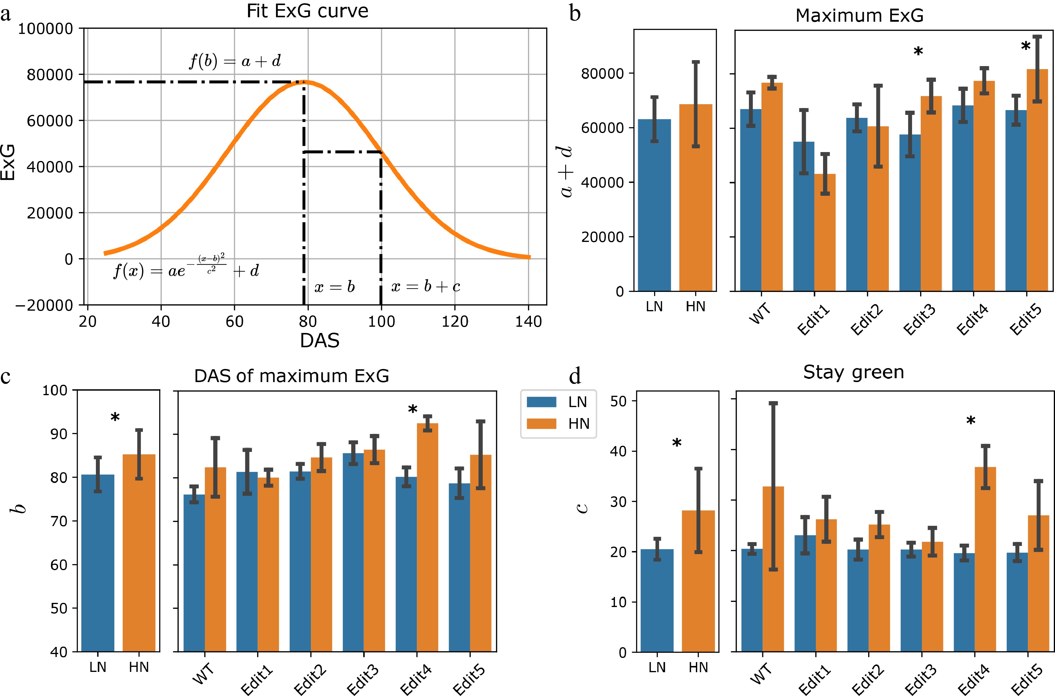
Figure 3. 

Modeling of the ExG index. (a) Fitting the ExG curve as a Gaussian curve and extraction of meaningful phenotypes. (b)−(d) The comparisons of the extracted phenotypes between N treatments. The left panel shows the overall comparisons between treatment and the right panel shows the comparisons for each genotype. The error bars indicate the standard deviation. Stars indicate a significant difference between low N and high N treatment for the pooled data or within a single genotype.

The b parameter revealed the DAS's maximum ExG. This specific date was achieved when the new growth of vegetation overtook the old vegetation's senescence, indicating the end of vegetative growth. The high N condition led to an overall significant (F-test, p-value = 0.016) later DAS to achieve the maximum ExG (Fig. 3c & Supplementary Table S6). The c parameter indicated the time between the DAS of the maximum ExG and the DAS of the maximum ExG growth or decay, which was defined as a measurement of the stay green phenotype (see Materials and Methods). A larger c parameter indicates the plant may stay greener for a longer time. Plants under high N generally stayed green for longer (F-test, p-value < 0.001). Per-genotype level significance for these two parameters was only observed in Edit4 (F-test, p-value = 0.001, Fig. 3d). Together with the maximum ExG and DAS of maximum ExG traits introduced above, these may suggest that sufficient N prolongs the plant's vegetation, while N deficiency might stimulate the plant to complete its reproductive cycle before resources are depleted.

Sustainable crop production is essential for ensuring food security for current and future generations. Improving nitrogen (N) use efficiency in plants is a key component of this goal, as excessive fertilizer use has significant environmental consequences. A deeper understanding of the nitrogen deficiency phenotype is critical for breeding crops with improved N utilization. Traditionally, biochemical methods such as measurements of chlorophyll or N content have been used to assess N status^[47]. While effective, these methods can be labor-intensive and less suitable for large-scale studies. Visual indicators like plant size and color offer a faster and more accessible alternative, but human-based assessments often lack precision. With the advancement of image-based high-throughput phenotyping, it is now possible to accurately and non-destructively measure plant traits at scale. The pixel count and ExG traits extracted from our study served as good close estimates of plant growth-related traits (Supplementary Fig. S6). In this study, a pipeline was developed to track the size and color of sorghum plants under varying nitrogen conditions throughout the developmental stages. To manage the high-dimensional temporal data, mathematical modeling approaches were employed to summarize growth and color trajectories into biologically meaningful parameters. These derived traits provided more interpretable and quantitative descriptions of N-related phenotypes, offering a robust framework for phenotyping N use efficiency. In total, five gene-edited sorghum lines were phenotyped under high N and low N environments in comparison to the Tx430 WT control. Tx430 WT demonstrated a growth-optimized strategy under high H compared to low N. It enriched chlorophyll content and accumulated the most biomass by taking full advantage of N resources. The edited lines showed compromised strategies with limited ability to capitalize on high N but significantly less than the WT. Edit1, especially with three N-related genes knocked out simultaneously, appeared to default to a stress phenotype, even when N resources were abundant. This may result from disrupted sensing or signaling pathways that fail to perceive high N as a growth-promoting cue; however, further investigations into the pathways in which each of the genes involved are needed.

This study introduced a new high-throughput phenotyping framework that discovered and quantified sorghum N-responsive traits. By estimating the parameters from the time-series growth curves, not only were the conventional end-point traits,such as above-ground biomass and N content, extracted, but also growth trajectory-related phenotypes. The model parameters in this study identified or derived several critical timings or stages. The treatments and phenotyping started on 29 DAS, on which the plants from both treatment groups were at the five-leaf stage (Fig. 1). As the N starvation progressed, sorghum exhibited different growth trajectories. The inflection point (µ) of pixel count and critical point (b) of ExG were likely related to the rhythm of the plant's growth, especially the transition between vegetative and reproductive growth. By examining the images from the experiment, the growth stage at the inflection point was estimated to correspond to growth stage 3, growing point differentiation^[48], and the critical point occurred at around the booting stage (Supplementary Fig. S7). The overall earlier occurrence of these critical timing under low N indicates the N effect that prolonged the increase in greenness or potentially the photosynthesis intensity^[49,50]. The third time point identified as important by the models was the time of the maximum decay of ExG (b+c). This may provide insights into the stay-green phenotype in response to N conditions. These are important in N response because in response to abiotic stresses, plants usually exhibit different strategies to balance the growth and stress response trade-off. Some plants may accelerate their maturity as a form of stress escape, while some may delay their maturity to accumulate the resources for successful reproduction^[51−53]. By looking at the growth and senescence rate, and the specific timing (such as inflection points in this study) in growth stages, clear differences were observed in the sorghum plants in response to N treatments. Moreover, identifying different growth trajectories improved the comparability of the two end-point traits since researchers traditionally select a specific date to measure all the plants, which may cause confounding results with the growth stage.

As high-throughput and high-intensity plant phenotyping develops, time series repeated measurements become increasingly achievable for researchers. This poses a challenge in developing appropriate models to analyze the phenotypic dynamics of plants. In this study, high-dimensional time-series traits were summarized into N-responsive phenotypic traits using two mathematical models. This approach modeled the plant growth trajectories with available measurements from the experiment. Compared to the approach that analyzes each single time point separately, the modelling approach used in this study is more statistically and biologically meaningful in incorporating information from nearby time points. It also reduces the post hoc efforts for interpretation after the single time point comparisons. There have been several attempts to address this problem using non-parametric functional models^[28−31]. Miao et al. ^[30] used a functional principal component (FPC) analysis to extract the main variations in the growth curve of the height of the sorghum and used FPC scores as phenotypes to identify genomic markers associated with the height of the plant. This method is effective in distinguishing between genotypes or treatments, but the interpretation of each FPC remains challenging without pre-annotated genetically associated data. Another non-parametric model, FANOVA, has also been applied to dissect the variance of genotypes and treatments^[28], but the resulting comparisons are represented as functional data and may present a challenge to understand. On the contrary, the mathematical modeling approach reduced the dimension of the time-series data to well-defined parameters, which can be directly linked to biological processes. It is also less prone to the hyperparameters of the model and the random noise in the growth curve. In addition, the resulting mathematical models are effective for predicting the unobserved phenotype of the plants. Along with the widely used sigmoid function for plant growth^[31,43,54], this study identified the ExG growth pattern as a Gaussian peak function with an additional vertical adjustment. This implied that, based on the pattern of the growth dynamic, various mathematical functions may be constructed or adjusted to describe the data. Despite several advantages of modeling the temporal phenotype with mathematical functions, it is worth noting that no model is correct. The mathematical models smooth the data based on functions that require prior assumptions. Important features might be lost if the assumptions misrepresent the data. It was observed that skewed Gaussian peak functions can better capture the unbalanced growth and decay rates of the ExG curves, but the additional parameter may introduce more uncertainty and difficulty in the biological interpretation of the parameters. This study presented the feasibility of a high-throughput temporal phenotyping pipeline for sorghum N-responsive traits. It is promising to be used in future studies, but more replication and careful experimental design will be required to boost the statistical power for accurate gene functional characterizations.