Research on the deployment model of intelligent highway sensor network under a bilevel programming framework

To confront the difficulties arising from the continuous growth in the number of vehicles, measures must be taken to enhance the safety and efficiency of road usage while minimizing its impact on the ecological environment. As a result, the concept of V2I cooperation has emerged. Nevertheless, as research progresses in autonomous vehicle technology, new challenges have also arisen. Integrating multiple sensor data to obtain information about the surrounding environment not only increases costs but also imposes greater demands on the data processing capabilities of decision support systems. Relying solely on a single autonomous vehicle to perceive the road conditions is insufficient to meet the standards of safe driving. Therefore, Intelligent Vehicle Infrastructure Cooperative Systems (IVICS)^[1] have emerged as a pivotal element in advancing the smart transportation sector.

In recent years, with the progress of autonomous driving technology, V2I cooperative systems have garnered widespread attention globally and have become a hot topic for research and development^[2−5]. For example, in the United States, the IntelliDriveSM program^[6] has been implemented to promote the development and application of vehicle-to-road cooperative technologies. In Europe, systems like eCall^[7] have facilitated swift information exchange between vehicles and traffic infrastructure in emergencies. The SmartWay initiative has been put into action in Japan^[8], incorporating a suite of advanced technologies including Advanced Highway Systems (AHS), Vehicle Information and Communication Systems (VICS), Automated Surveillance Vehicles (ASV), and Electronic Toll Collection (ETC). In combination, these systems enhance roadway safety and mitigate traffic jams.

Vehicle clustering is a key technology for analyzing and optimizing traffic flows in Intelligent Transportation Systems (ITS)^[9]. By effectively grouping vehicles, the dynamic characteristics of traffic flow can be better understood, providing decision support for traffic management, congestion mitigation, and environmental monitoring. With the continuous development of urban traffic data collection techniques, research on vehicle clustering methods has also been evolving and improving. In terms of data-driven clustering algorithms, Ryu et al.^[10] proposed a clustering algorithm based on dynamic spatiotemporal correlation to predict traffic flow, achieving good prediction accuracy by training the prediction model with historical data. In the field of behavioral pattern clustering algorithms, Choong et al.^[11] used KMeans and FCM clustering algorithms to evaluate the clustering performance of driver vehicle trajectories under different parameters, selecting the optimal solution. In the realm of multi-source data integration, Gao et al.^[12] have introduced a novel hybrid routing algorithm that leverages the Time-Elastic Band (TEB) approach. This algorithm offers enhanced precision for navigation systems that rely on mapping and has the potential to supersede conventional manual-guided autonomous mapping techniques. In the direction of dynamic clustering, Mohri et al.^[13] constructed an improved Measure of Cumulative Accessibility (MCA) using real-time travel demand information. Additionally, deep learning-based clustering analysis has also gained significant attention. Wang et al.^[14], for example, utilized machine learning-based clustering algorithms to cluster vehicle trajectories based on learned vehicle vectors, thereby improving trajectory prediction accuracy.

RSUs are critical components in ITS, deployed alongside roads to communicate with vehicles, provide traffic information, support safety applications, and facilitate vehicle automation. Proper RSU deployment is essential for achieving effective V2I communication. In the realm of coverage area evaluation, Feng et al.^[15] delved into the deployment and enhancement of vehicular communication networks. They introduced a heuristic method contingent on density, ensuring the fulfillment of coverage demands while markedly cutting down on equipment costs, thus bolstering the security and dependability of vehicular communication networks. Economic viability is equally important, and Degrande et al.^[16] assessed the financial aspects of C-ITS RSU deployment through the lens of road management, comparing the capital outlay with anticipated gains to minimize expenses. Furthermore, concerning dynamic deployment tactics, Ali Almazroi et al.^[17] introduced a budget-efficient method for the dynamic placement of RSUs, contingent on the density of road traffic, ensuring line-of-sight (LOS) connectivity between the RSU and cellular network.

This paper has two main innovations: first, based on the requirements of intelligent highway sensor network construction, an innovative RSU deployment model has been constructed, which comprehensively considers the factors of coverage benefits, information transmission deficiencies, construction, and maintenance costs. The constructed RSU optimization layout model is used for visual analysis, analyzing the variations of the model under different scenarios. Second, in the aspect of information transmission deficiencies, an optimized model is innovatively established by adding constraints to the energy consumption model, aiming to minimize the flooding time and maximizing the energy efficiency of the intelligent highway sensor network. This effectively limits excessive network energy consumption, achieving the goal of energy savings and optimizing the RSU deployment model.

Within the framework of a smart highway sensing network that facilitates interactions through both peer-to-peer vehicle communication and infrastructure-to-vehicle communication protocols, this study formulates an enhanced RSU placement strategy. The strategy is crafted from the vantage point of those responsible for the intelligent highway sensing network, taking into account a cost-benefit analysis. This includes the advantages of RSU's roadside information reach, the potential for data transmission degradation over time, and the associated expenses of deployment and upkeep^[18,19]. The model calculates the optimal spacing for deployment in various penetration rate scenarios to minimize the expenses associated with the installation. This study, grounded in the interplay of traffic dynamics and information flow theories^[20−24], and the energy depletion model of Wireless Sensor Network (WSN) nodes^[25], revises the model to incorporate the characteristics of penetration rates. It assesses the necessary adjustments in RSU deployment, specifically the spacing, in response to varying profit conditions.

Analysis of roadside RSU perception under vehicle-road cooperative perception

V2I networks primarily consist of RSUs, On-Board Units (OBUs), and communication networks, including V2V, V2I, and V2X (Vehicles and Everything) communication. In V2I networks, V2V and V2I are crucial for information exchange^[26,27], and RSUs serve as the hub for information interaction. The deployment of RSUs directly impacts the quality of the V2I network. Nevertheless, focusing solely on V2I communication leads to heightened deployment expenses due to the necessity of a high concentration of RSUs. Additionally, it introduces the challenge of information interference among these units, which can lead to the transmission of superfluous vehicle data.

Currently, research on RSU deployment in the academic community does not consider the impact of penetration rate, i.e., the proportion of smart cars relative to the overall vehicle count. Conventional deployment schemes often account for communication range and the costs associated with deployment, yet they frequently neglect the implications of deploying intelligent connected vehicles that serve as conduits for information transfer. When RSUs engage with nearby intelligent connected vehicles, those within the RSU's coverage area can relay information seamlessly. Vehicles positioned beyond the coverage area can still facilitate V2I communication by leveraging intermediate vehicles, thus significantly expanding the reach of information distribution, as depicted in Fig. 1. Furthermore, influenced by the performance of the devices and external environmental factors, existing wireless communication technologies may encounter issues with delayed or ineffective information transfer, particularly when the devices are spaced too far apart. Consequently, in planning the placement of RSUs, it is essential to determine optimal spacing to ensure efficient information transfer. Suitable spacing can maximize the efficiency of information transmission. Furthermore, due to the relatively simple scenarios on highways, which are conducive to autonomous vehicles operating according to rules, most intelligent highway pilot projects are based on highway scenarios. In this study, the highway is chosen as the research scenario.

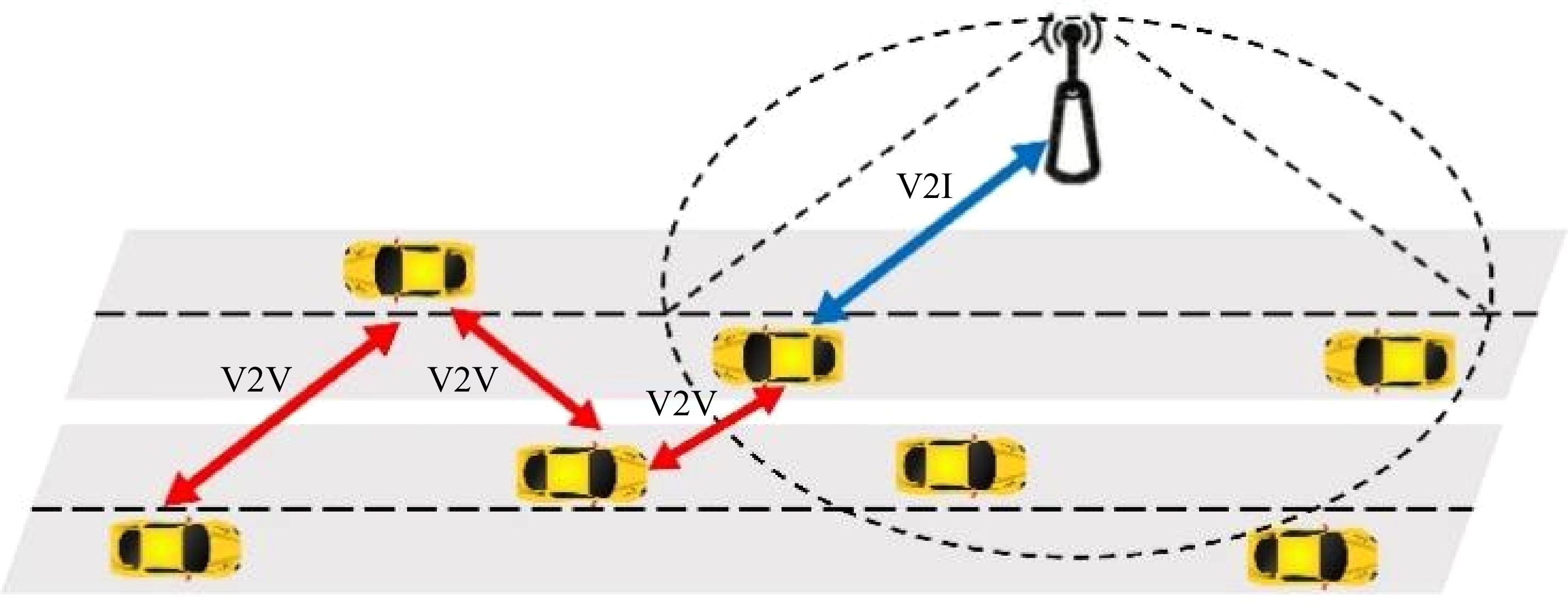
Figure 1. 

Diagram of information transmission in vehicle-to-infrastructure cooperative systems.

Basic theory of the layout model

In vehicular ad hoc networks, numerous smart connected vehicles function as nodes for information dissemination, playing a crucial role in network communication. While various scholars have delved into the positioning of vehicles within road networks, analyzing the specific motion characteristics of individual vehicles is impractical due to their high velocities, the complexity of predicting their paths, and the sheer volume of nodes involved. Hence, this study focuses on vehicle clusters as the subject of investigation within vehicular ad hoc networks. In this study, a vast fleet of vehicles is consolidated into unified groups, enabling intra-cluster information exchange via both direct and relayed (multi-hop) communication methods. Given the sparse traffic, swift vehicle movement, consistent travel paths, and foreseeable motion patterns on expressways, the Poisson distribution is an appropriate model. The occurrence of vehicles in proximity to roadside detection systems on highways is presumed to adhere to a Poisson distribution. In other words, the likelihood of observing n vehicles over a stretch of road L, given a certain average traffic flow λ, is depicted by the formula presented in Eqn (1).

Cars are assumed to arrive according to a Poisson process, with the intervals between arrivals conforming to an exponential pattern. Given the premise that the studied vehicles travel at uniform speeds, it is inferred that the spacing X between them is distributed exponentially, as illustrated by Eqn (2). Under the hypothesis that the communication radius of smart vehicles form a circular area with a radius of Rv, the likelihoods of communication and lack thereof between vehicles within and beyond this range are delineated by Eqns (3) and (4), respectively.

Here, α represents the penetration rate. Inside a vehicular cluster, every constituent node is capable of receiving the messages disseminated by the cluster's leader. Accordingly, the extent of a vehicular cluster can be ascertained by evaluating the number of intervals present. The likelihood of encountering intervals within a cluster is delineated by Eqn (5).

Drawing from the principles of the coupling between information and traffic flow, the dissemination of information in a connected vehicular network can be categorized into two distinct modes: immediate dissemination and relay-based propagation. When the distance between adjacent vehicles does not exceed the radius of information dissemination, an immediate transfer of data takes place, with the message being conveyed directly from one vehicle to another via wireless transmission. Otherwise, the mechanism of relay transmission is activated. In this scenario, the information becomes mobile, traveling alongside the vehicles as they move with the flow of traffic. During the relayed transmission, the pace of information dissemination is synchronized with the vehicle's speed, continuing until the gap to the next intended vehicle aligns with the communication radius. Once the relay transmission is concluded, it initiates a fresh cycle of information dissemination.

Consequently, the dissemination of information within vehicular traffic adheres to a consistent sequence, where each information cluster consists of one or more immediate transmissions along with a single relay transmission. Let X denotes the distance covered in immediate transmission, Y denotes the distance for relay transmission, and E denotes the length of the vehicle cluster; thus, the total transmission distance L for a set of information can be calculated by combining these two components. Owing to the variability inherent in dynamic traffic conditions, the distances for both types of transmission are subject to randomness. By considering the distribution of distances between vehicles in traffic, the average distances for these two modes of transmission can be derived, as illustrated in Eqn (6).

Fundamental presumptions

(1) The lifespan of information, denoted as τ in this paper, is established as a set parameter. If the period required for a vehicle to relay information to the RSU via multi-hop surpasses the information's inherent lifespan, further transmission is halted, resulting in the loss of the information's currency. Moreover, it is posited that the affirmative advantages gained by each category of vehicle post-reception of information are consistent.

(2) In this paper, the vehicle clusters are composed of vehicles that travel in a specified direction, aligning with the orientation of the road. The length of each road segment is set at 1,000 m, featuring an average traffic density of λ and an average traffic speed of $\overline v $ .

(3) Each intelligent vehicle node has a fixed and identical transmission radius. Relative to the data transmission speed, the vehicles are in a relatively stationary state and are randomly distributed in a rectangular area as a static network. Intelligent vehicle nodes use data packets of fixed lengths for data transmission. Within extensive sensor networks, the following two special cases are ignored: ① Intelligent vehicle nodes use the minimum transmission radius to ensure network connectivity; ② Intelligent vehicle nodes use the maximum transmission radius to cover the entire network.

(4) In expansive sensor networks, the costs associated with the deployment, upkeep, and power supply for each RSU and the proprietary network is established and recognized. The unit cost remains unaltered regardless of changes in the deployment span; hence, the total expenditure is exclusively determined by the changes in distance^[28].

(5) Direct connections are forged among RSUs, with the wiring length being equivalent to the gap between these RSUs. The study does not encompass the wired linkage between RSU and the cloud platform^[28].

This section further explores the correlation between the penetration rate and various factors including the benefits of RSU information coverage is denoted by C_cov(α), the degradation of information transfer throughout its lifespan indicated by C_L(α), as well as the expenses related to the establishment and upkeep denoted by C_P(α). For C_cov(α), concerning the link between the penetration rate and the coverage scope, grounded in the prevailing theory of traffic and information flow integration, this paper will delineate this connection and formulate the function for the benefits of RSU information coverage. For C_L(α), addressing the correlation between the penetration rate and the decay incurred by information transmission throughout its lifespan, this paper will construct it based on the Wireless Sensor Network (WSN) node energy consumption model. For C_P(α), regarding the cost, under the condition of unchanged unit prices for equipment installation and maintenance, the cost is only related to the installation quantity and deployment length of RSU, which can be directly used for calculation. Therefore, the optimized deployment model of RSU, Max-Perm (Maximization of Profit through Permeability), is expressed as Eqn (7). When smart highway builders attach importance to the impact of energy consumption on information transmission, they can control the size of α₁ to affect the overall revenue. At this time, builders need to re-plan the spacing and use positive revenue to compensate for the information energy consumption caused by vehicle communication in the highway. Similarly, when smart highway builders attach importance to the impact of construction costs, they can control the size of α₂ to affect the overall revenue. Builders also need to re plan the spacing and use positive benefits to offset some of the construction costs of the highway:

where, α₁ and α₂ represent the loss coefficient and cost coefficient, respectively, used to control the dimensional effects among distinct entities.

Advantages of RSU information reach

As vehicles travel on highways and intelligent connected vehicles are introduced, drivers receive increased surrounding information, resulting in more stable driving, approximating homogeneous traffic flow. The assumption is that the vehicle's velocity is v_i and the subsequent vehicle's velocity is v_i ± Δv_n.

Under assumption (1), within the information lifecycle τ, the advantages that accrue to each category of vehicle upon information reception are uniform. As a result, the benefits provided by the RSU's reach are directly proportional to the total number of vehicles affected by the spread of information. The advantage derived from each instance of information transmission corresponds to the highest count of vehicles reached by the information during its entire lifespan.

To accomplish this objective, this study initially develops a model for the length of vehicle clusters under varying penetration rates, drawing on the principles of the traffic flow-information flow interplay^[20−24]. Furthermore, in light of assumption (2), considering the situation of oncoming traffic flow, it constructs a model for the expected time of information transmission within the lifecycle. By merging the model of cluster dimensions, the model of anticipated timing, the reach of the RSU's coverage, and the density of average traffic flow, the overall count of vehicles within the coverage can be determined, denoted as C_cov(α).

Development of immediate transmission frameworks across varied penetration rates

The freeway context examined in this paper can be simplified to a linear representation. Inside the vehicular ad hoc network, intelligent vehicles serve crucial roles as information dissemination hubs, as shown in Fig. 2. When the distance between adjacent vehicles does not exceed the smart connected vehicles' detection radius R_v, direct transmission is initiated, facilitating immediate information exchange among vehicles wirelessly.

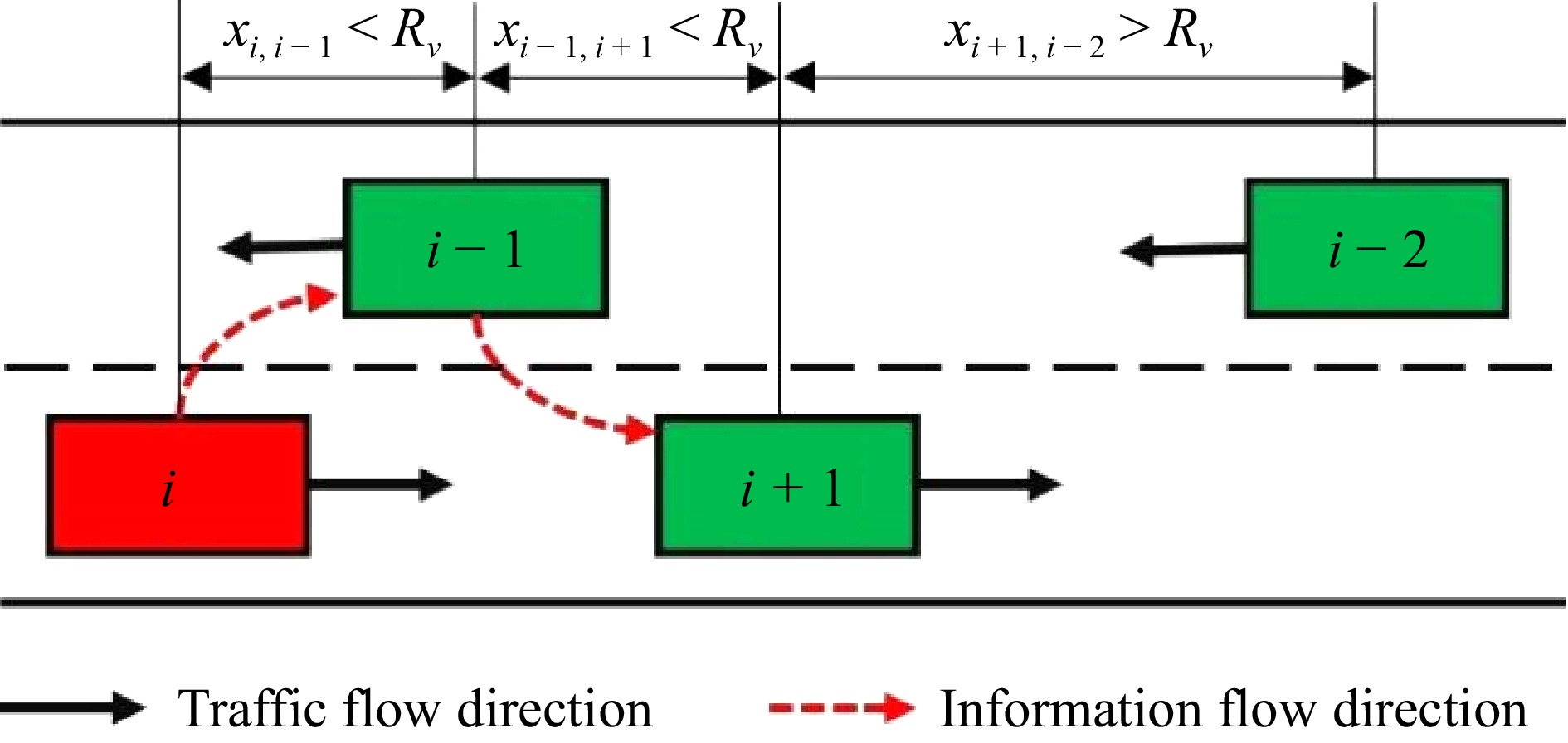
Figure 2. 

Instantaneous transmission.

In Fig. 2, should the distance x_i,i−1 between Vehicle i and Vehicle i−1, and the distance x_{i−1,i +1} between Vehicle i−1 and the following Vehicle i+1, both be less than the threshold R_v, the information from Vehicle i can be transferred to Vehicle i+1 in two phases, with Vehicle i−1 acting as a relay. If the separation between neighboring vehicles is greater than R_v, a relay transmission is initiated, with the vehicle transporting the information along the traffic flow until it reaches a point where the distance to the next intended vehicle is R_v. It is at this juncture that a new cycle of instantaneous transmission is initiated.

Throughout the information dissemination process, when the distance x is less than R_v, an immediate exchange of information takes place between vehicles. In line with the previously discussed characteristics of vehicle clusters, the projected distance for a one-step direct transmission is specified in Eqn (8), the span for the direct transmission itself is outlined in Eqn (9), and the duration required for the transmission is presented in Eqn (10):

In this context, $\overline k $ represents the projected number of relays needed for a group of information to facilitate immediate transmission, P indicates the probability of such immediate exchange occurring between vehicles, with their respective formulas provided in Eqns (11) and (12). τ_α is indicative of the time required for a single relay's transmission.

Development of models for relayed communication across diverse infiltration rates

When engaged in the relay transmission process, the data carried by the smart connected vehicles travels along the flow of traffic until the gap x reaches R_v, initiating the exchange of information at that juncture. Drawing on the principles of traffic flow-information flow interrelation, the relay transmission is categorized into four distinct modes, as illustrated in Fig. 3. Modes I and II commence from an identical starting condition, with the direction of traffic flow aligning with the direction of information dissemination, as depicted in Figs 3a and b. In Fig. 3a, the instance where Vehicle i passes Vehicle i+1 traveling in the same direction, before the approach of an oncoming Vehicle i−1, is designated as Mode I relay transmission. In Fig. 3b, the event where Vehicle i initially meets oncoming Vehicle i−1 is identified as Mode II relay transmission. In Modes III and IV, the direction of relay transmission is contrary to the direction of information flow, as depicted in Figs 3c and d. In Fig. 3c, Vehicle i, when overtaken by Vehicle i+1 moving in the same direction, exemplifies Mode III relay transmission. In Fig. 3d, as the distance between neighboring vehicles increases, Vehicle i must complete the information transfer before any meeting occurs, thereby switching to Mode II relay transmission.

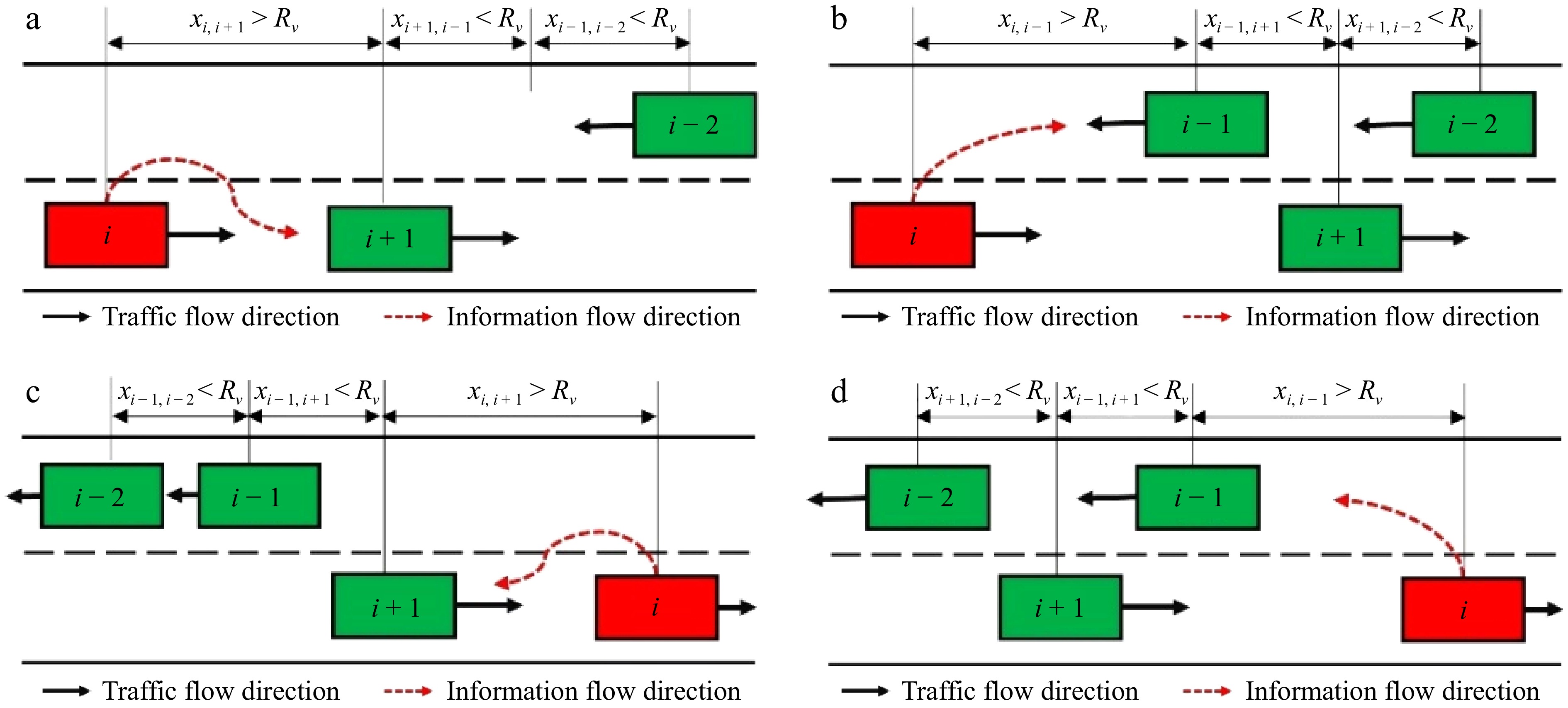
Figure 3. 

Four modes of relay transmission. (a) The first type, (b) the second type, (c) the third type, and (d) the fourth type of ferry transportation.

Consequently, these four aforementioned modes are grouped into three unique transmission classes. When deriving the anticipated transmission distance E(Y) for relay transmission, it is ascertained by integrating the weights of these three distinct transmission modes, as delineated in Eqns (13) and (14), complemented by the corresponding transmission timing outlined in Eqn (15):

Here, E(Y_n) denotes the anticipated transmission distance across the aforementioned trio of modes, β_n signifies the relative share of these modes, v_i is indicative of the velocity of vehicles conveying information, and Δv_n corresponds to the speed of pursuing vehicles.

Vehicle count under RSU influence across various penetration levels

Based on the earlier examination, the conveyance of information within the traffic flow is divided into direct and relayed transmissions. By calculating the ratio between the distance of transmission and the time taken for transmission, one can infer the pace at which a batch of information spreads throughout the traffic flow, as demonstrated in Eqn (16). Consequently, the scope of information distribution, L, throughout its lifespan τ, is defined by Eqn (17). The reach of RSU in terms of vehicle coverage, that is, the affirmative advantages, is articulated in Eqn (18).

where, R represents the RSU coverage radius.

Adverse impacts stemming from information dissemination loss

In the formulation of the adverse impact model, the detrimental effects primarily include the loss of information transmission C_L(α) and the expenses associated with the construction and maintenance of the wired network C_P(α). Within this section, a quantitative account of the issue grounded in assumption (3) is provided, employing the energy expenditure on node information transmission to symbolize the economic detriment C_L(α) due to information distortion, followed by a detailed explanation.

Higher-tier planning model and network flooding time

In the sphere of V2V and V2I interactions, the network flooding time and network energy consumption will become hotspots and focus of large-scale wireless sensor network research. When intelligent connected vehicles transmit information in a smart highway sensor network, flooding, a robust method is usually used to send data packets to surrounding nodes.

However, traditional flooding propagation not only consumes a large amount of energy but also occupies the entire network's communication channel for a long time. Consequently, drawing from the examination of how the transmission radius of smart vehicles influences the flooding duration and the impact of packet length on the energy expenditure of sensor networks, a two-tiered programming structure is suggested. The goal of the higher-tier model (U) is to set the optimal intelligent vehicle sensing radius to minimize the flooding time, thereby achieving the fastest data packet transmission speed. The subordinate model (L), influenced by the upper-level model, seeks the optimal packet length to maximize the efficiency of the smart highway sensor network, aiming to reduce the drawbacks of traditional flooding propagation.

Higher-tier model (U): The network flooding time consists of receiving time T_R and contention channel time T_C. The reception duration represents the mean interval for network nodes to acquire broadcast packets, whereas the contention channel duration denotes the mean interval for nodes to both receive and transmit data packets. In addition, the setup time T_S denotes the mean duration it takes for all network nodes to disseminate flood packets, that is T_S = T_R + T_C.

T_R varies directly with the sensor network's area S and inversely with the transmission radius R_v of the smart vehicles. Therefore, considering the effect of packet length on T_R, Eqn (19) is derived.

where, k₁ is a constant factor. When the sensor network area contains α × n smart connected vehicles, the number of neighbor nodes $\overline m = {\text π} \dfrac{{{R^2}}}{{{S^2}}}\alpha n$ and the corresponding contention channel time T_C are given by Eqn (20), where k₂ is another constant factor. The constructed upper-level planning model is shown in Eqn (21).

In the higher-tier model (U), there are two unknown variables R_v and L_P(L_P = l + α_P). The higher-tier model (U) can only control the variable R_v while L_P is passed from the subordinate model (L) to the upper-level model as a known variable. Therefore, the upper-level model seeks to minimize the flooding time in the sensor network by finding the optimal R_v under a given packet length L_P.

Subordinate planning model and network efficiency

Subordinate model (L): A data packet generally consists of a header α_P, payload l, and tail τ. The header usually contains information such as time, location, and events, while the payload includes valid information collected by sensor nodes. The tail includes error control codes. When data packets do not use error control codes but only CRC checks, it can be approximated τ = 0.

The energy consumed by a single hop during the transmission of information between nodes can be divided into energy consumed by non-transmitting devices E_ele, energy consumed by transmitting devices ${E_{amp}} = \dfrac{{\beta {R_v^r}}}{{{\eta _{amp}}}}$, and energy required to receive information E_rx. β is a hardware constant, which becomes a fixed value when the sensor type is determined. r is the path attenuation factor, η_amp is the transmitter gain. Total energy consumption E_total includes two parts: multi-hop transmission energy E_data and energy required for control packets E_control. Therefore, the expression for single-hop transmission energy E_1hop is given by Eqn (22).

In addition, when the payload length of the data packet is ρ, the energy required for control packets E_control when transmitting n_bit bit data is given by Eqn (23).

Based on Eqn (23), when transmitting $n$ bit data, the total energy consumption ${E_{total}}$ is given by Eqn (24).

In the sensing network, when the information is transmitted in the channel, there are certain information will exist error phenomenon, at this time, the probability of correctly receiving the data packet is ${\left( {1 - {p_e}} \right)^{l + {\alpha _p}}}$, p_e is the burst error rate, which is generally calculated using empirical Eqn (25).

To maximize the energy efficiency of data transmission, the subordinate model (L) is given by Eqn (26).

In the subordinate model (L), the unknown variables are R_v and L_P, but the subordinate model can only control the variables L_P and R_v are parameters passed down from the higher-tier model (U), which are known variables. Therefore, for a given transmission radius R_v, the information transfer deficit C_L(α) = E_total(R_v,L_P) is determined by finding the optimal packet length L_P to minimize the energy loss in the transmission process.

Adverse effects of infrastructure development and maintenance expenses

Within the third domain of the construction and upkeep expenditure C_P(α), it is further segmented into two components: the expenses for the wired network and those for the roadside RSUs. In accordance with assumption (4), the per-unit expense for the wired network necessary for the installation of RSUs is established and unvarying; it remains constant irrespective of an increase in the deployment span. The deployment length of the wired network is employed to denote a detrimental cost. Assumption (5) posits that RSUs are interconnected by direct lines, arranged in a linear formation down the center of the road in a straight alignment.

In calculating the expenses for construction and maintenance C_P(α), the area depicted in Fig. 4 serves as the foundation for computation. Thereafter, the expense of the wired network for this segment is classified into two scenarios contingent on the length of the cluster, as specified in Eqn (27). When E(C) < R, the information exchange between vehicle clusters as depicted in Fig. 4a does not extend the communication range of the RSUs. In such instances, C_P(α) is solely associated with R. When E(C) > R, the information relay between vehicle clusters as illustrated in Fig. 4b is capable of augmenting the communication reach of RSUs, and this is correlated with both C_P(α) and E(C). In conclusion, the expense for the wired network is calculated by multiplying the span of the RSU reach and the extent of individual vehicle clusters across various segments by the unit cost of the wired network. The aggregate expenditure is the aggregate of the wired network expenses and the outlay for the RSU, as indicated in Eqn (28).

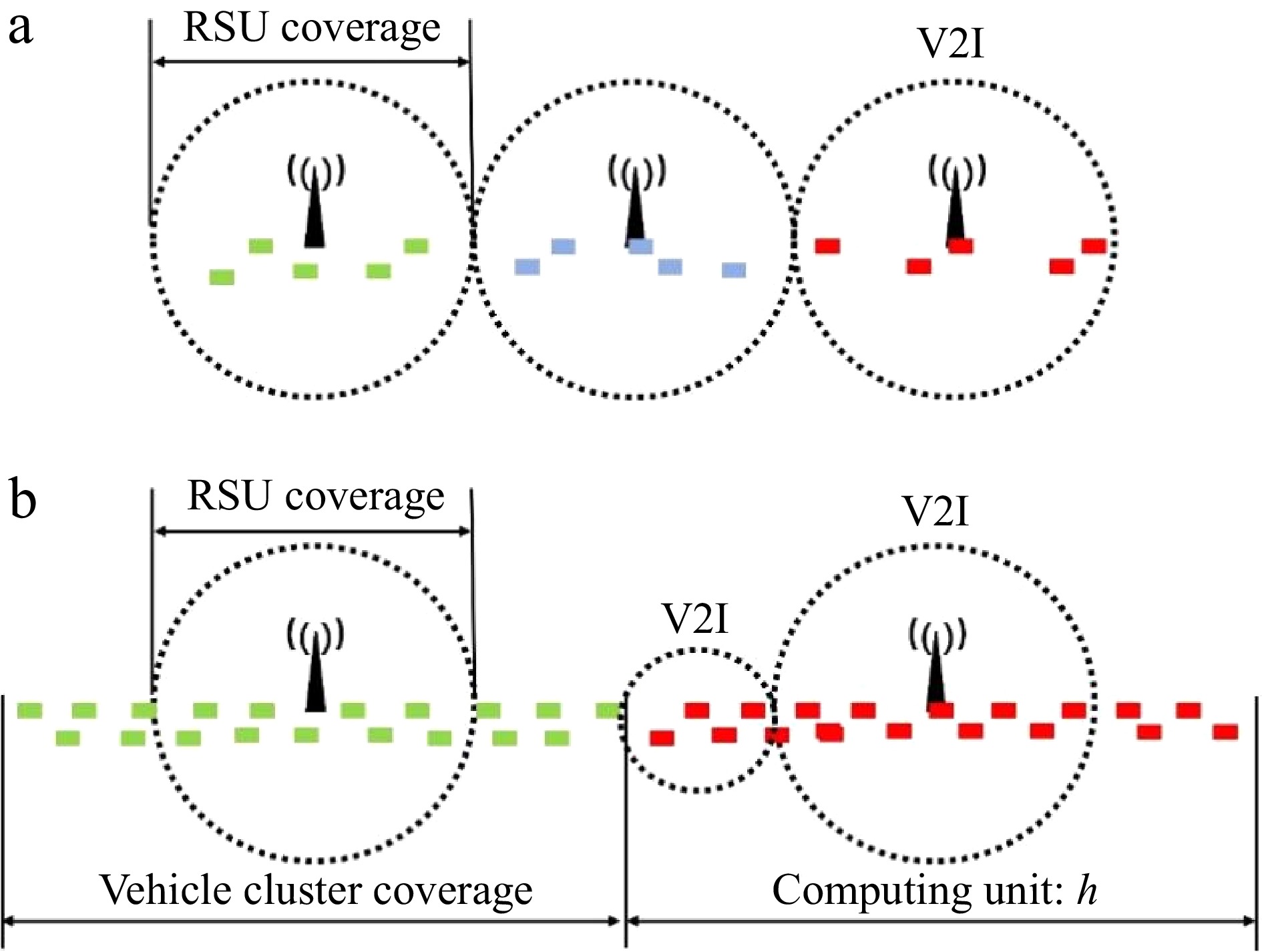
Figure 4. 

RSU calculation unit. (a) E(C) < 2R, (b) E(C) > 2R.

In this context, the span of an individual vehicle cluster is E(C), the count of computational units is h, the per-unit expense for the wired network is γ, and the per-unit cost of the RSUs is η.

The MATLAB experimental simulation platform, equipped with capabilities for data analysis, fulfills the investigative demands of this study. Employing MATLAB to develop the model for optimal placement referred to as Max-Perm, in the S = 0.04 × 1 km² highway space, simulate different traffic density, with the increasing penetration rate of the gain how to change, scrutinize the pivotal points within the revenue fluctuation graph, to determine the value of the gain under the different objectives can be inversely deduced under the corresponding purpose of the layout spacing, to achieve the layout spacing under different layout purposes.

In the section dedicated to affirming the positive gains from coverage by RSUs, a model for verifying network connectivity is applied to confirm the V2V connection rate once efficient information transfer is established among clusters. Within the segment addressing the validation of information transmission deficits, the power exhaustion of system components is evaluated under varying traffic scenarios and infiltration quotas using the optimized KMeans clustering approach.

The parameter settings for the optimization layout model Max-Perm are shown in Table 1.

Empirical findings and quantitative assessment

Iterative analysis of two-level planning models

According to Adverse Impacts Stemming from Information Dissemination Loss's Negative return model under information transmission deficiency, combined with Laboratory Configuration and Parameter Allocation's parameter setting, the higher-tier model (U) and subordinate model (L) are analyzed by MATLAB software with the following heuristic algorithm:

Step 1: Set an initial solution ${R_v^0}$, making the number of iterations k = 0;

Step 2: For the specified ${R_v^0}$, address the subordinate model (L) to derive l^k;

Step 3: Integrate L_P = α_P + l^k into the responsive function and calculate the revised ${R_v^{k + 1}}$ value;

Step 4: Stop if $\left| {T_S^{k + 1} - T_S^k} \right| \leqslant \varepsilon $, where ε = 0.05;

Alternatively, let k = k + 1, and proceed to step 1, where ε is the iteration precision.

The outcomes of the bi-level planning model's iterations are presented in Table 2.

Within the framework of a two-level planning challenge, the key goal is to establish the responsive function of the lower-tier issue concerning the dominant problem L_P(R_v), and by embedding this functional linkage into the higher-level model, the model's optimal solution, indicated by ${R_v^*}$, can be resolved. As the upper-level planning model (U) in this paper is very special, it is an unconstrained planning problem, if it is solved, it can be made $\dfrac{{d({T_S})}}{{d{R_v}}} = 0$, at this time, we can obtain Eqn (29), where N = α × n.

In Table 2, the model uses different initial values of transmission radius (R₀ = 50, 100, 150 200) for the iterative computation, and when the range enters into the extreme value range, all of them can achieve the same optimal solution ${R_v^*}$ = 63.8478. It can be seen that this heuristic algorithm solution is able to converge to the optimal solution. At this point, the optimal solution ${R_v^*} $ = 63.8478 is brought into Eqn (29), and the optimal transmission packet length L* = (16 + 15.9993 = 32 byte can be obtained.

Optimized layout model analysis

In this segment, MATLAB is employed to render the model's visualization, as depicted in Fig. 5a, where curve L1 represents the function's peak trajectory. As traffic congestion on the highway increases progressively, the summit curve nears the surface linked to an infiltration rate of zero. In other words, as traffic density grows and hits its zenith, the necessary penetration rate diminishes. Curve L2 signifies the boundary path, when this curve is surpassed by a point on the surface, it signifies a positive return for the model; conversely, if the point is below the curve, it indicates a negative return. Curve L3 illustrates the formation of inter-vehicle connectivity at its onset. As the density of traffic flow escalates, the state curve, upon reaching its peak, demands a reduced penetration rate. An increase in traffic flow density thus corresponds to a decreased necessity for penetration rate, particularly at the curve's peak, as observed in Fig. 5b. It is evident from the same figure that within region S3, no vehicle-to-vehicle connectivity will emerge.

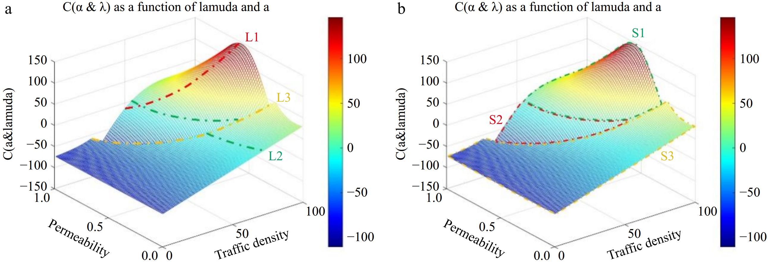
Figure 5. 

3D surface diagram of the Max-Perm model.

By capturing a profile of the scenario amid heightened traffic density, Fig. 6a illustrates these three key nodes, a, b, and c, on the curve. Node a marks a stage where the penetration rate is still low, with benefits primarily driven by the negative aspect of deployment costs. Beyond node a, vehicles start to establish connections, and concurrently, the proliferation of smart networked vehicles amplifies the positive benefits derived from the RSU's information coverage. This progression continues until the point b is reached, marking the transition to a positive benefit margin. Nevertheless, with the escalation of the penetration rate, the overall energy expenditure on information exchange between nodes correspondingly rises, which in turn restricts the curve's ascent. Upon reaching point c, the adverse effects outweigh the positive gains, prompting the benefit curve to descend, signifying that the model has reached its peak condition at this juncture.

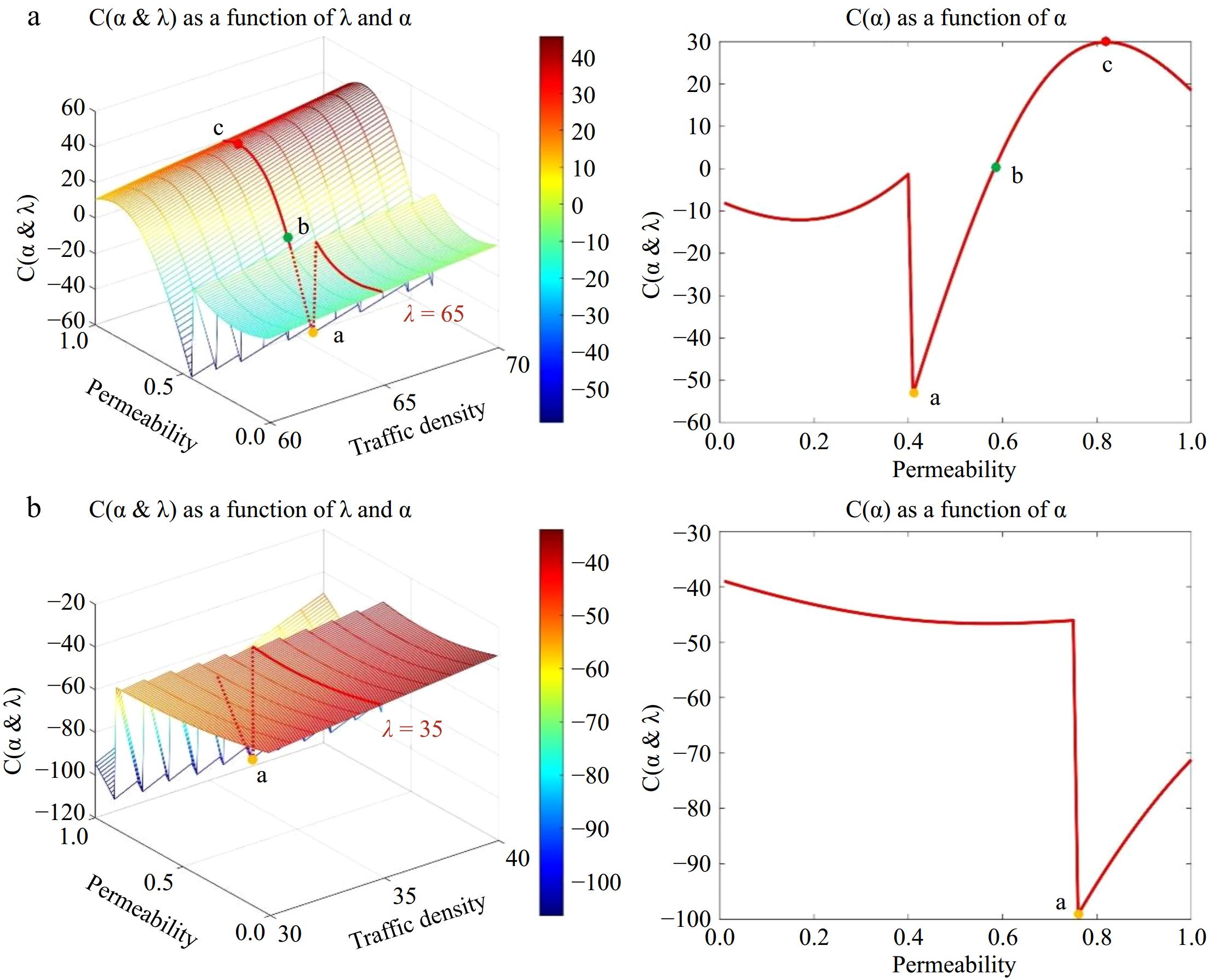
Figure 6. 

Variation of slices for high and low density models.

Capturing a cross-section of the model's surface at a low traffic density, as illustrated in Fig. 6b, discloses a solitary crucial node a on this curve, in contrast to Fig. 6a, and its value is negative. At this level of traffic density, irrespective of increases in the penetration rate, the model's deployment cost remains negative, suggesting that an optimal deployment interval does not exist under these circumstances.

Simulation verification

In the section analyzing the forward coverage gains of RSUs, the Warshall algorithm simulation is implemented to substantiate the model's dependability. Within a simulated area of 40 m × 100 m, vehicle nodes numbering 40, 60, 80, and 100 are dispersed at random. In each network scenario, a subset of nodes is randomly designated to function as the intelligent grid vehicles, and with an increasing count of designated smart grid vehicles, the penetration rate escalates in tandem. At this juncture, the respective networks initiate connectivity at penetration rates of 26%, 29%, 41%, and 69%. As depicted in Fig. 7b these rates closely align with the values at node a in the Iterative Analysis of Two-level Planning Models mentioned earlier, which mark the onset of interconnectivity between the models, as illustrated in Fig. 7a.

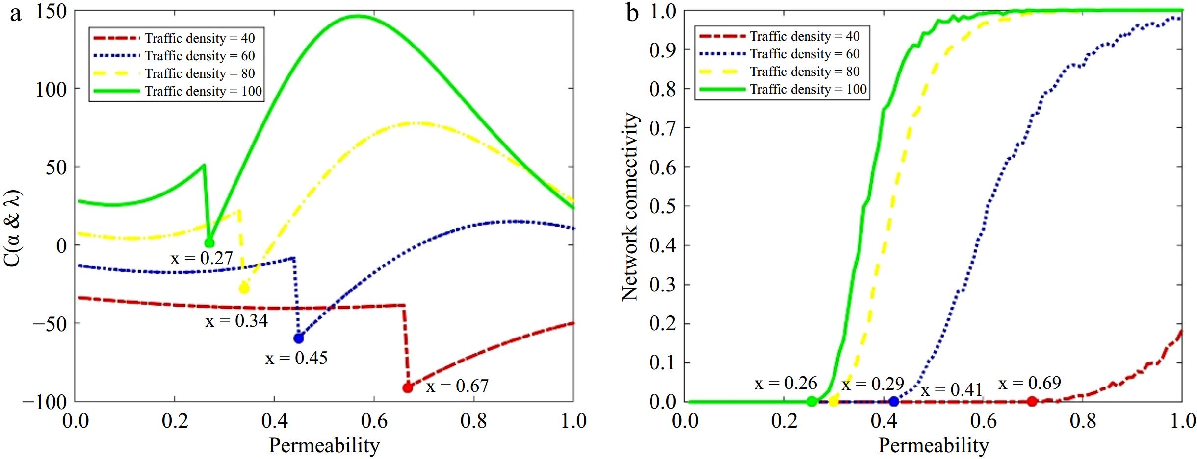
Figure 7. 

Positive benefit simulation verification.

In the segment dedicated to the deficiency test of information transmission, the model's reliability is confirmed through simulation using the cluster-based routing protocol. The model's performance at a traffic density of 100 is validated, as indicated by the red curve in Fig. 8a. Within a simulated area measuring 40 m × 100 m, 100 vehicle nodes are dispersed at random, with subsets of 20, 40, 60, and 80 nodes being arbitrarily chosen to represent smart connected vehicles. The depletion due to information exchange among nodes is emulated with a clustering algorithm, yielding outcomes of 15.650, 31.739, 47.879, and 63.379, as illustrated in Fig. 8b, aligning closely with the model's projected values.

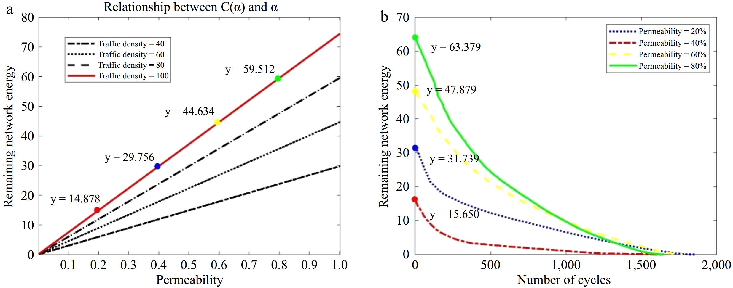
Figure 8. 

Information transmission loss simulation verification.

In summary, the results and effects from the model's validation stage are detailed in Tables 3 and 4.

Tackling the deployment necessities for RSUs within a vehicular-cooperative framework, this study presents a superior strategy for RSU positioning in a setting where V2V and V2I communications intersect. Analyzing the revenue model's dynamics, influenced by penetration rates and traffic flow density, through the lens of an intelligent highway sensor network constructor, the paper identifies the penetration values for various revenue scenarios. Consequently, this approach allows for the calculation of the spacing along the roadway for each scenario. Furthermore, the dependability of each model component is substantiated through simulations using the Warshall algorithm and cluster routing protocols. The central conclusions drawn here involve:

(1) A revenue framework for smart highway sensors, influenced by the integration of connected vehicles, is proposed. By scrutinizing the outcomes of revenue equations across various penetration rates and traffic densities, the optimal spacing for RSUs under these conditions is ascertained. For instance, considering a traffic density of 80:

Scenario 1: When the intelligent networked vehicles reach 34%, the vehicles begin to form an effective connection between them, that is, when they are located on the state curve L3, at this time, the length of vehicle clusters is 132 m, which is smaller than the sensor sensing radius of 200 meters, and at this time, the spacing of the deployment of the 2 × R that is, 400 m;

Scenario 2: Upon attaining a 40% threshold of smart grid vehicles, the revenue model equates to zero. In this instance, the vehicle cluster's length is measured at 169 m, falling short of the 200-m sensor detection radius. Consequently, the deployment interval is set at 2R, equating to 400 m;

Scenario 3: As the proportion of smart grid-connected vehicles grows and hits 69%, the revenue model achieves its maximum value, coinciding with the summit of curve L1. In this scenario, the vehicle clusters span 554 m, exceeding the 200-m sensory range of the sensors. Consequently, the deployment spacing is determined to be 2R + E(C) , that is, 554 m, indicating the revenue model's optimal state.

(2) Simulation using the Warshell algorithm verifies the penetration rate of vehicles wanting to form an effective connection when the density of traffic flow is 40, 60, 80, 100. Moreover, the simulation outcomes indicate that the constructive benefit segment possesses a reliability of 92.451%. Using the cluster routing algorithm simulation to verify the traffic density of 100, the penetration rate of 20%, 40%, 60%, 80%, the information transfer of the resulting defect, simulation results show that the information transfer of the defective part of the reliability of 93.985%.

In conclusion, given that the model development and simulation both employ a homogeneous traffic flow, the benefit model offers a high degree of reliability in ascertaining the placement intervals within a freeway context, rendering it apt for directing the strategic placement of RSUs.

Constraints and prospects for further inquiry

Initially, the model presented in this paper takes into account solely the deficits in information transmission and the expenses for construction and maintenance within the negative benefit component, without exploring the safety concerns potentially stemming from the loss of connectivity among networked vehicles. The article posits that any vehicle experiencing disconnection will be corrected by the driver for malfunctions, and that such anomalies will not impact the surrounding traffic during the rectification. Therefore, safety concerns should be integrated into future research to avert any potential accidents caused by malfunctioning vehicles.

Secondly, the model was developed within a highway context that is relatively free from external factors, and it does not account for disruptions caused by inclement weather; subsequent studies ought to consider the impact of detrimental environmental conditions.