







-
Unmanned aerial vehicles (UAVs) play an increasingly important role in scenarios such as patrol prevention, video tracking, high-altitude positioning, vehicle tracking, and target identification[1−5], significantly enhancing social and security services[6−8]. However, small and medium UAVs are limited by size and weight and therefore typically take off via hand-launch or ejection, often using folded fixed wings for a high lift-to-drag ratio. A typical sequence is: the UAV is packaged inside the launcher, propelled out by high-pressure gas, after which the V-tails and wings deploy to achieve fixed-wing flight (Fig. 1).
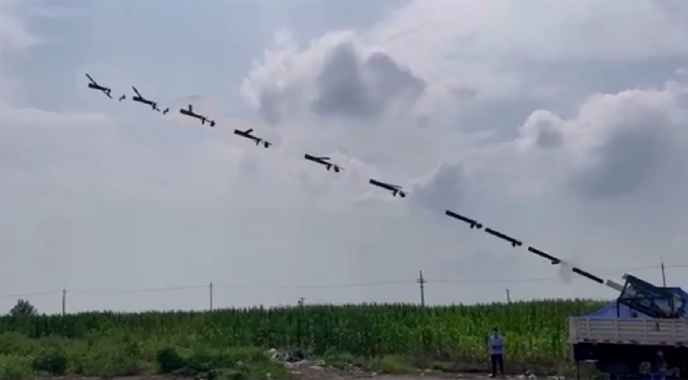
Figure 1.
Flight experiment of the launch process of this paper.
In this sequence, the launch phase is the most dynamically severe and failure-prone stage of the whole mission chain: the high overload at the launch instant can exceed the sensor range; wall friction can induce post-exit autorotation; wing/tail deployment introduces abrupt aerodynamic and inertia changes; and the propulsion motor produces reaction torque at startup. These factors are superimposed within an extremely short time window, placing stringent demands on the real-time disturbance-rejection capability of the control system. Disturbance rejection and stabilization tailored to the launch phase are therefore key to the mission success rate of gun-launched UAVs and form the focus of this paper.
Launch system
-
A gun/tube launch system typically comprises the launch tube, a high-pressure gas or gas-generator unit, in-tube guidance and restraint mechanisms, and a release mechanism. The launch timeline can be summarized as: (i) the high-pressure gas accelerates the folded UAV to the required muzzle velocity within an extremely short time (accompanied by high launch overload); (ii) the UAV exits the tube and the restraint is released; (iii) the V-tails and then the wings deploy; (iv) the propulsion motor is unlocked and started, establishing fixed-wing flight. This timeline corresponds one-to-one with the control-strategy time nodes see T0–T4 in section Control strategy for the launch process.
Designing the autopilot for such a variable-geometry vehicle requires handling the following problems:
• Initial launch dynamics: the sudden acceleration during catapult launch can exceed the sensor range, causing velocity errors that the algorithm must compensate for to stabilize the UAV quickly.
• Friction-induced rotation: friction between the UAV and the launcher wall can cause autorotation on exit, which must be corrected immediately for a stable, controlled trajectory.
• Wing and tail deployment: the dramatic aerodynamic changes from deployment introduce model disturbances affecting lift, drag, and stability.
• Propulsion-motor activation: motor startup exerts an undesirable reaction torque on attitude that the control system must counteract.
• Aerodynamic variability, center-of-gravity shift, high-speed control response, sensor calibration, and environmental factors must also be handled by robust control.
Contribution
-
Both traditional and modern control approaches have been studied for variable-geometry platforms. Adaptive control, such as L1 adaptive control combined with dynamic inversion, has been applied to variable-sweep morphing aircraft to handle configuration-induced nonlinearities and maintain tracking performance over a wide flight envelope[9];
$ H_\infty $ Besides the proposed scheme, nonlinear model predictive control (NMPC) is widely applied to control platforms with uncertainties. Although it can handle system constraints, NMPC involves massive online optimization calculations and obvious time delays, which cannot satisfy the fast response requirements during the launch phase of GL-UAVs. In comparison, active disturbance rejection control (ADRC) aggregates uncertain dynamics into a lumped total disturbance, which is estimated and compensated in real time by an extended state observer (ESO). ADRC delivers fast tracking and strong disturbance rejection, requires no precise system model, and boasts simple design and implementation[13−16]. Recently, the combination of hierarchical sliding mode control and control barrier functions has been applied to constrained attitude stabilization of underactuated systems.
Over the past 5 years, ADRC and its core components, the ESO and the
$ {\rm{fal}}(\cdot) $ Based on this comparison, this paper adopts a cascaded ADRC built around the ESO, because its combined advantages in robustness, disturbance rejection, fast response, model independence, and design simplicity best fit the engineering needs of the GL-UAV launch phase.
The main contributions of this work are as follows:
• Disturbance rejection for launch-phase transients: a cascaded ESO-based angular-rate stabilizer specifically handles abrupt aerodynamic and inertia changes during fold-to-deploy and the motor-startup reaction torque, markedly improving disturbance rejection over conventional algorithms.
• Segmented throttle control (novel engineering contribution): segmented slow acceleration suppresses motor-startup reaction torque, reducing the measured peak roll rate from 0.42 to 0.26 rad/s (about 38%) so the system meets the launch-success criteria.
• Clear and reproducible launch-success criteria: the subsection Criteria for the successful launch process gives quantitative criteria (e.g., roll rate converging to ± 0.05 rad/s within 1.5 s after full throttle), providing an objective, reproducible benchmark for similar gun-launched/catapult UAVs.
-
In this paper, we introduce a small variable-geometry UAV characterized by a low-wing and V-tail configuration. As shown in Fig. 2, both the wings and V-tails can be folded. The wings fold below the fuselage, while the V-tails fold along the sides of the fuselage. The parameters of the UAV system are described using the following abbreviations: RI for rotational inertia, UN for undeployment, and DE for deployment.
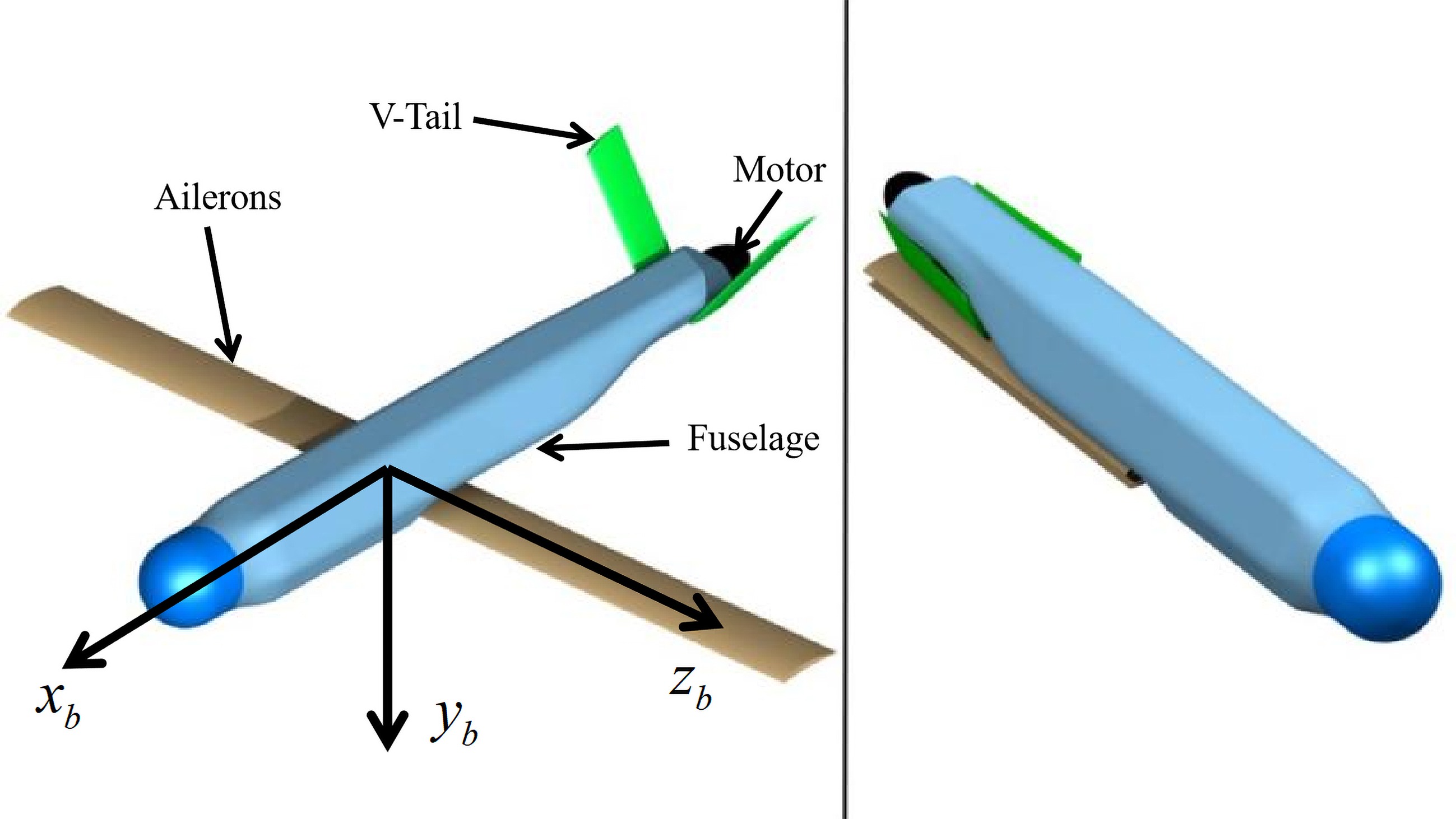
Figure 2.
The layouts of small variable-geometry UAV: left side, wings unfolded; right side, wings folded.
• Weight (kg): 13
• Wing span (m): 0.2 (UN), 1.9 (DE)
• Reference area (m2): 0.02 (UN), 0.22 (DE)
• Launch air pressure (MPa): 2.3 (UN), 2.3 (DE)
• RI of body
$ x_b $ • RI of body
$ y_b $ • RI of body
$ z_b $ We define the body-fixed frame
$ x_b $ $ y_b $ $ z_b $ $ \begin{aligned}\left\{\begin{aligned}C_x & =C_x\left(V,\alpha,\beta,\delta_e\right) \\ C_z & =C_z\left(V,\alpha,\beta,\delta_e\right) \\ C_y & =C_y\left(V,\alpha,\beta,\delta_a,\delta_r\right) \\ L & =L\left(V,\alpha,\beta,\delta_a,\delta_r\right) \\ M & =M\left(V,\alpha,\beta,\delta_e\right) \\ N & =N\left(V,\alpha,\beta,\delta_a,\delta_r\right)\end{aligned}\right.\end{aligned}. $ (1) Here,
$ \alpha $ $ \beta $ $ \delta_a $ $ \delta_e $ $ \delta_r $ The aerodynamic coefficients are obtained from Computational Fluid Dynamics (CFD) simulations and stored as interpolation (look-up) tables, which are evaluated online as functions of airspeed, angle of attack, sideslip angle, and control-surface deflections.
The roll, pitch, and yaw channels are represented by the virtual inputs
$ \delta_a $ $ \delta_e $ $ \delta_r $ The nonlinear model contains forces, moments, kinematics, and navigation and can be organized as in[6,7].
The deformation dynamics of a projectile-launched transformable UAV are governed by a set of equations that describe the forces, moments, and motions involved during the transformation process. These equations include
Aerodynamic forces and moments:
$ \begin{aligned} {\bf{F}}_{{\rm{aero}}}=\dfrac{1}{2}\rho V^2 S\,{\bf{C}}_F\left(\alpha,\beta,\delta_e,\delta_a,\delta_r\right), \end{aligned} $ (2) $ \begin{aligned} {\bf{T}}_{{\rm{aero}}}=\dfrac{1}{2}\rho V^2 S\,{\bf{C}}_M\left(\alpha,\beta,\delta_e,\delta_a,\delta_r\right), \end{aligned} $ (3) where,
$ \rho $ $ {\bf{C}}_F\in\mathbb{R}^{3\times 1} $ $ {\bf{C}}_M\in\mathbb{R}^{3\times 1} $ $ \alpha $ $ \beta $ Control forces and moments are computed from
$ \delta_a $ $ \delta_e $ $ \delta_r $ Rotational motion equations:
$ \begin{aligned} {\bf{I}}\dfrac{d{\boldsymbol{\omega}}}{dt}+{\boldsymbol{\omega}}\times\left({\bf{I}}{\boldsymbol{\omega}}\right)={\bf{T}}_{{\rm{ext}}}, \end{aligned} $ (4) where,
$ {\bf{I}}\in\mathbb{R}^{3\times 3} $ $ {\boldsymbol{\omega}}\in\mathbb{R}^{3\times 1} $ $ {\bf{T}}_{{\rm{ext}}}\in\mathbb{R}^{3\times 1} $ The kinematic relationship between the pitch angle
$ \theta $ $ \begin{aligned}\dot{\theta}=q\cos\phi-r\sin\phi\end{aligned}, $ (5) where,
$ \phi $ It projects body-frame rates onto the inertial attitude rate and is the bridge between the outer attitude loop and the inner angular-rate loop in the cascade: the outer loop generates a rate command from the attitude error, and the inner loop tracks it.
Translational motion equations:
$ \begin{aligned} m\dfrac{d^2{\bf{r}}}{dt^2}={\bf{F}}_{{\rm{ext}}} , \end{aligned} $ (6) where, m is the mass of the UAV,
$ {\bf{r}}\in\mathbb{R}^{3\times 1} $ $ {\bf{F}}_{{\rm{ext}}}\in\mathbb{R}^{3\times 1} $ The translational motion equations are retained in the full dynamic model for two main reasons. First, flight velocity, angle of attack, and sideslip angle, which are essential for calculating aerodynamic coefficients in Eq. (6), are derived from translational states. Second, these equations are used to calculate launch overload and reproduce the ballistic trajectory during the gun-launch phase. Since the proposed controller only focuses on attitude and angular-rate regulation without velocity/position closed-loop control, translational dynamics do not appear in the control block diagram, but are still necessary for high-fidelity simulation.
Deformation equations:
$ \begin{aligned} {\bf{M}}\dfrac{d^2{\bf{u}}}{dt^2}+{\bf{C}}\dfrac{d{\bf{u}}}{dt}+{\bf{K}}{\bf{u}}={\bf{F}}_{{\rm{int}}}, \end{aligned} $ (7) where,
$ {\bf{u}}\in\mathbb{R}^{3\times 1} $ $ {\bf{M}}\in\mathbb{R}^{3\times 3} $ $ {\bf{C}}\in\mathbb{R}^{3\times 3} $ $ {\bf{K}}\in\mathbb{R}^{3\times 3} $ $ {\bf{F}}_{{\rm{int}}}\in\mathbb{R}^{3\times 1} $ $ {\bf{F}}_{{\rm{int}}} $ These equations must be solved simultaneously to accurately predict the UAV's behavior during launch, transformation, and subsequent flight. Advanced numerical methods and simulations are often employed to analyze these dynamics and ensure reliable performance.
Control strategy for the launch process
-
Before launch, the wings and V-tails are folded and loaded into the launcher (Fig. 3). High-pressure gas first pushes the UAV out of the tube, after which the wings and V-tails deploy and the propulsion motor is activated. As shown in Fig. 4, the specific control strategy for the launch process is listed as follows:
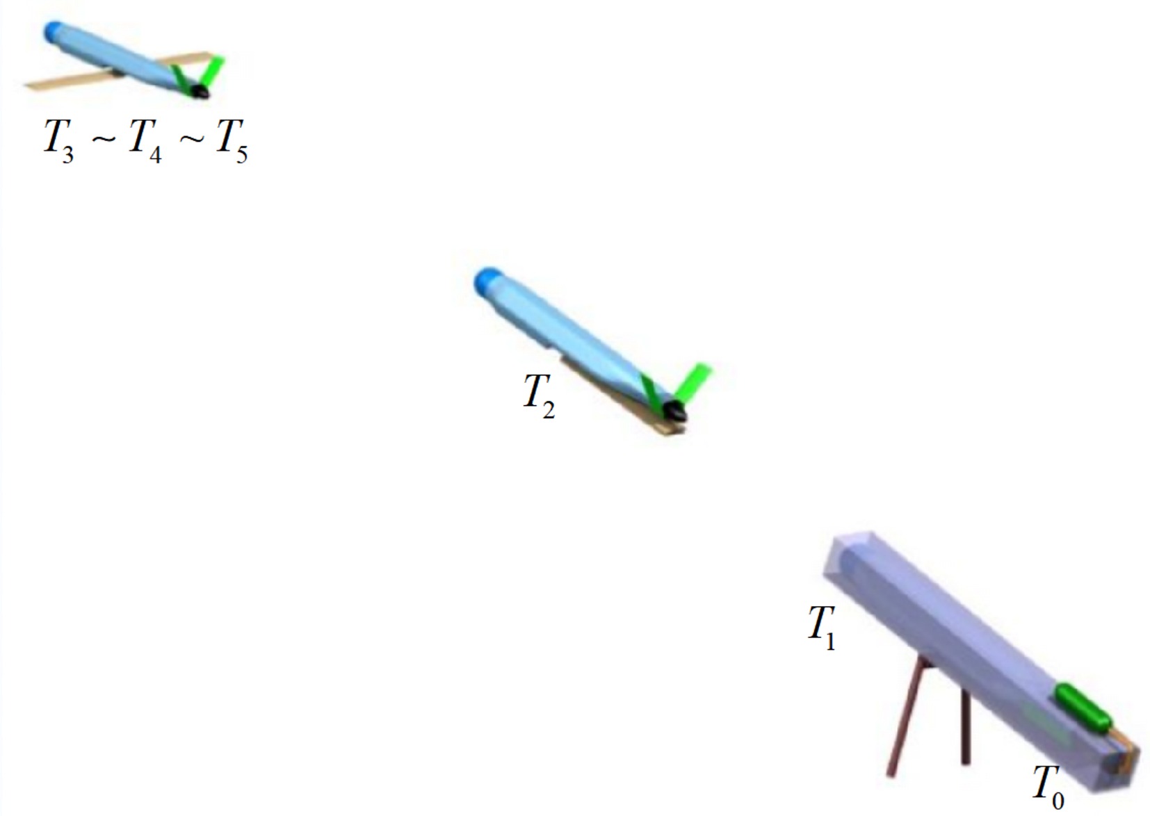
Figure 3.
Animation of launch process.
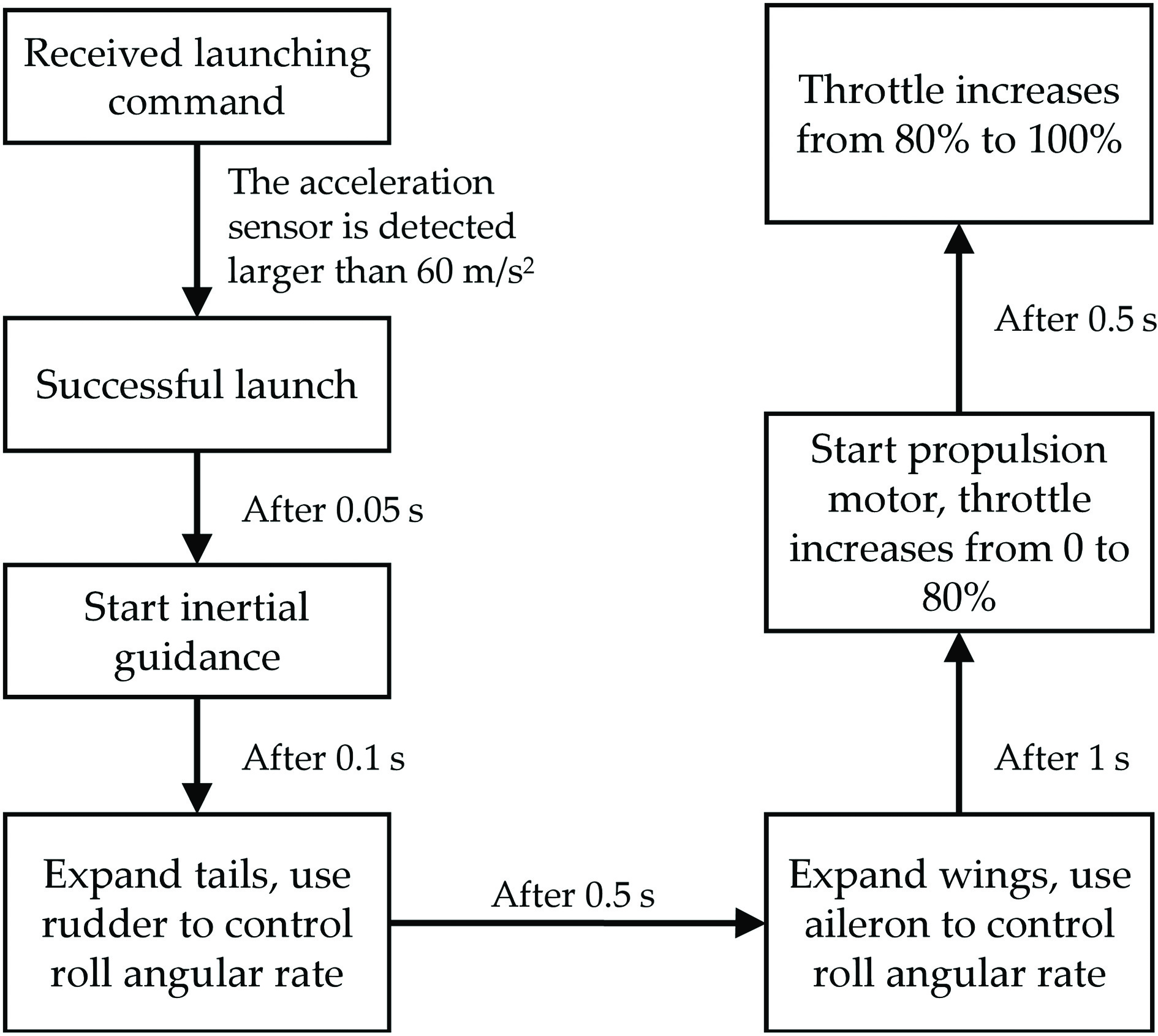
Figure 4.
Control strategy for the launch process. High-pressure gas firstly pushes the UAV out of the launcher, and then the wings and V-tails deploy and the propulsion motor is activated.
• When the autopilot receives the launch command, high-pressure gas pushes the vehicle out of the tube; this instant is denoted as T0. The in-tube propulsion rapidly accelerates the UAV to the required initial speed. The inertial measurement unit (IMU) continuously measures the
$ x_b $ • T1: the IMU estimates the vehicle's velocity and angular rate; the velocity is determined by integration from the launch velocity.
• T2: the V-tails deploy. The elevator maintains the pitch angle at 5° (launch angle), and the rudder suppresses roll by regulating the roll rate to 0°/s. Immediately after launch, the trajectory is approximately parabolic; to minimize longitudinal maneuvering, the pitch command is set to follow the tangent of the parabola.
• T3: the wings deploy. The ailerons regulate the roll rate to 0°/s, while the elevator maintains the pitch angle at 5°.
• T4: the propulsion motor is activated. To mitigate propeller reaction torque, a segmented slow-acceleration strategy is adopted: the throttle increases from 0% to 80% gradually, and then increases from 80% to 100% approximately 0.5 s later. After reaching 100%, the throttle is held for 4 s before entering the acceleration phase.
Cascaded control design
-
A cascaded ADRC attitude controller is adopted to stabilize the launch process. The attitude dynamics are separated into a fast inner loop (angular rate) and a slow outer loop (attitude angle), and the control gains are tuned according to the timescale-separation principle. Given the actuator reconfiguration during launch, the virtual control inputs
$ q_c $ $ p_c $ 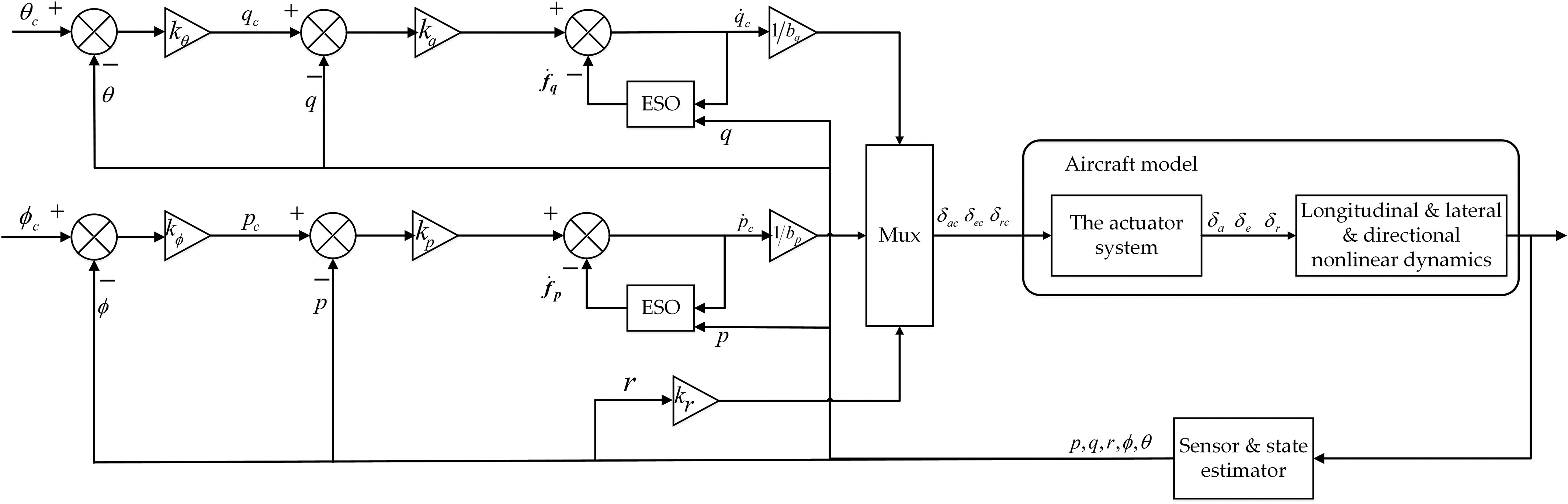
Figure 5.
Complete control architecture. Pitch and roll cascaded ESO-based control schemes to handle the control stabilization.
The designed cascaded controller aims to stabilize UAV attitude and angular rate during launch, so independent velocity feedback control is not adopted. The translational motion model is reserved to describe force-moment coupling and support numerical verification, rather than participating in real-time control.
Cascaded longitudinal control
-
The pitch angle rate command
$ \dot{\theta}_c $ $ \begin{aligned} \dot{\theta}_c = k_{\theta}\,\bigl(\theta_c-\theta\bigr), \end{aligned} $ (8) where,
$ k_{\theta} $ $ \begin{aligned}q_c & =\dfrac{1}{\cos \left(\phi\right)}\, \dot{\theta}_c+r\, \sin \left(\phi\right)\end{aligned}. $ (9) Taking the derivative of both sides of Eq. (9), we obtain
$ \begin{aligned}\ddot{\theta}\approx\dot{q}\cos\phi+q\dot{\phi}\sin\phi-\dot{r}\sin\phi-r\dot{\phi}\cos\phi\end{aligned}\ \ . $ (10) By rotational dynamics,
$ \begin{aligned} \dot{q} = \dfrac{M-pr\left(I_x-I_z\right)}{I_y} \end{aligned} $ (11) where, p is the roll angular rate and Ix, Iy, and Iz are the rotational inertias.
Combining Eqs (10) and (11), the dynamics can be written as
$ \begin{aligned}\ddot{\theta}=f_q+M_{\delta_e}\, \delta_e\end{aligned}, $ (12) where, M denotes the total pitch moment,
$ M_{\delta_e} $ $ \begin{aligned}f_q & =-\dot{r}\sin\phi-r\dot{\phi}\cos\phi+q\dot{\phi}\sin\phi \\ & \quad+\dfrac{M-\left(I_x-I_z\right)pr}{I_y}\cos\phi-M_{\delta_e}\, \delta_e\ .\end{aligned} $ (13) Define
$ y_q=\dot{\theta} $ $ x_{1q}=\dot{\theta} $ $ x_{2q}=f_q $ $ \begin{aligned}\left\{\begin{aligned}\dot{x}_{1q} & =x_{2q}+b_q\, \delta_e\ , \\ \dot{x}_{2q} & =w\ , \\ y_q & =x_{1q}\ ,\end{aligned}\right.\end{aligned} $ (14) where,
$ b_q=M_{\delta_e} $ To reduce the phase delay, a second-order nonlinear ESO is used in the pitch angular rate control loop:
$ \begin{aligned}\left\{\begin{aligned}e_{1q} & =z_{1q}-y_q, \\ \dot{z}_{1q} & =z_{2q}+b_qu_q-\beta_{1q}e_{1q}, \\ \dot{z}_{2q} & =-\beta_{2q}\, \rm{fal}(e_{1q},\alpha,\delta),\end{aligned}\right.\end{aligned} $ (15) where,
$ z_{1q} $ $ z_{2q} $ $ \beta_{1q} $ $ \beta_{2q} $ $ {\rm{fal}}(\cdot) $ $ \begin{aligned} {\rm{fal}}(e_{1q},\alpha,\delta)=\begin{cases} \dfrac{e_{1q}}{\delta^{1-\alpha}}, & |e_{1q}|\leqslant\delta,\\ |e_{1q}|^{\alpha}\operatorname{sign}(e_{1q}), & |e_{1q}| \gt \delta. \end{cases}, \end{aligned} $ (16) where, the sign function is defined as
$ \begin{aligned} \operatorname{sign}(x)=\begin{cases} 1, & x \gt 0,\\ 0, & x=0,\\ -1, & x \lt 0. \end{cases} \end{aligned} $ (17) The observer parameters satisfy
$ \alpha\in[0,1] $ $ \delta $ $ \operatorname{sign}(\cdot) $ $ {\rm{fal}}(\cdot) $ $ \begin{aligned} \left\{\begin{aligned} s &= \dfrac{\operatorname{sign}(e_q+\delta)-\operatorname{sign}(e_q-\delta)}{2},\\ {\rm{fal}}(e_q,a,\delta) &= \dfrac{e_q}{\delta^{1-a}}s+|e_q|^a\operatorname{sign}(e_q)(1-s). \end{aligned}\right. \end{aligned} $ (18) With a given parameter of
$ {\rm{fal}}(\cdot) $ $ \delta $ $ a $ $ {\rm{fal}}(e_q,1,\delta)=e_q $ $ a $ $ \begin{aligned} {\rm{fal}}(e_q,0,\delta)=\begin{cases} \operatorname{sign}(e_q), & |e_q| \gt \delta,\\ \dfrac{e_q}{\delta}, & |e_q|\leqslant\delta. \end{cases} \end{aligned} $ (19) In this case,
$ {\rm{fal}}(\cdot) $ Combining the nonlinear ESO in Eq. (14), the estimation error can be constructed as
$ \begin{aligned} \left\{\begin{aligned} e_{2q} &= z_{2q}-x_{2q},\\ \dot{e}_{1q} &= e_{2q}-\beta_{1q}e_{1q},\\ \dot{e}_{2q} &= -\beta_{2q}\,{\rm{fal}}(e_{1q},\alpha,\delta)-w. \end{aligned}\right. \end{aligned} $ (20) The pitch angular rate control law is
$ \begin{aligned}u_q=\dfrac{u_{0q}-z_{2q}}{b_q}\end{aligned}, $ (21) where,
$ u_{0q} $ $ \begin{aligned}u_{0q}=k_q(q_c-q)\end{aligned}, $ (22) where, kq represents the bandwidth of the pitch angular rate loop. From Eq. (12), the original plant can be tuned to a pure integrator plant, and the closed inner-loop transfer function can be reorganized as
$ \begin{aligned}\dfrac{\omega(s)}{\omega_c(s)}=\dfrac{k_q}{s+k_q}\end{aligned}. $ (23) Cascaded lateral-directional control
-
Similar to the pitch channel, the roll dynamics can be written as
$ \begin{aligned}\dot{p}=f_p+L_{\delta_a}\, \delta_a\end{aligned}, $ (24) where,
$ f_p $ $ \begin{aligned}f_p=\dfrac{(I_y-I_z)I_z}{I_xI_z}rq+\dfrac{I_z}{I_xI_z}L-L_{\delta_a}\, \delta_a\end{aligned}, $ (25) where,
$ L_{\delta_a} $ • Significant changes happen in Ix and aerodynamic moments from folding to deployment states.
• A relatively high gyroscopic moment is caused by the motor at its activation window.
The roll angular rate control law is
$ \begin{aligned}u_p=\dfrac{k_p(p_c-p)-z_{2p}}{b_p}\end{aligned}, $ (26) where,
$ b_p=L_{\delta_a} $ $ \begin{aligned} \left\{\begin{aligned} e_{1p} &= z_{1p}-y_p,\\ \dot{z}_{1p} &= z_{2p}+b_p u_p-\beta_{1p}e_{1p},\\ \dot{z}_{2p} &= -\beta_{2p}\,{\rm{fal}}(e_{1p},\alpha,\delta). \end{aligned}\right. \end{aligned} $ (27) The vehicle's deployable state shows a pronounced Dutch roll mode. To simplify the yaw channel control design, only damping stabilization is implemented. The damping control law can be organized as
$ \begin{aligned}u_r=k_r\, r\end{aligned}. $ (28) The closed-loop stability analysis, including observability and controllability, can be referred to in Benyahia et al.[5].
Determination of ESO/fal(·) parameters and generalization
-
The ESO gains
$ \beta_1 $ $ \beta_2 $ $ \omega_o $ $ \beta_1=2\omega_o $ $ \beta_2=\omega_o^2 $ $ \omega_o $ The
$ {\rm{fal}}(\cdot) $ $ \alpha$ $ \delta $ $ \alpha $ $ \delta $ Thanks to this parameterization, porting the proposed scheme to another gun-launched UAV only requires re-selecting
$ \omega_o $ $ \delta $ $ \alpha $ -
The launch process is simulated by MATLAB/Simulink. Three artificial disturbances are introduced into the simulation:
• The spontaneous rotation caused by the friction between the UAV and the launcher's wall is simulated when the vehicle is launched out of the tube.
• The disturbance caused by the deployment of the wings is simulated. The V-tail is close to the fuselage, and the disturbance to the vehicle can be ignored.
• The torque caused by motor activation is also simulated.
The amplitudes and time histories of these roll-moment disturbances are not heuristic but are identified from measured flight data of the launch process, so that the simulated disturbances reproduce the magnitude and characteristics of the real launch environment. For the present vehicle, the equivalent roll-moment disturbances are on the order of a few N·m, which is consistent with the post-launch attitude excursions observed in the flight tests. This data-driven setting ensures that the conclusion that the proposed controller can cope with realistic disturbances is supported by representative disturbance levels rather than by artificially conservative ones.
Disturbance simulation model and parameter settings of inner-loop control
-
The trimming point is set at an airspeed of 36 m/s and an altitude of 50 m. The second-order systems with position and rate limitations are matched to the actuators. The characteristics of the actuators are: the aileron, elevator, and rudder have a natural frequency of 8 Hz, a damping ratio of 0.8, a position limitation ± 25°, and a position rate limitation ± 100°/s, as shown in Table 1. We design the ADRC controller abiding by the following control specifications:
Table 1. Characteristics of the actuators.
Actuator Natural
frequency (Hz)Damping
ratioPosition
limitation (°)Position rate
limitation (°/s)Aileron 8 0.8 ± 25 ± 100 Elevator 8 0.8 ± 25 ± 100 Rudder 8 0.8 ± 25 ± 100 • Level 1 flying qualities.
• Time-delay margin greater than 100 ms.
• Gain margin greater than 6 dB.
• The static error of the step response is within 0.05.
The ESO-related control parameters are shown in Table 2.
Table 2. ESO-related control parameters.
Parameter Value ESO fal function, $ \alpha $ 0.5 ESO fal function, $ \delta $ 0.01 Pitch angular rate ESO gain, $ \beta_{1q} $ 20 Pitch angular rate ESO gain, $ \beta_{2q} $ 100 Roll angular rate ESO gain, $ \beta_{1p} $ 20 Roll angular rate ESO gain, $ \beta_{2p} $ 100 Bandwidth of pitch inner-loop, $ k_q $ 6 Bandwidth of roll inner-loop, $ k_p $ 10 Bandwidth of pitch outer-loop, $ k_{\theta} $ 1.5 Bandwidth of roll outer-loop, $ k_{\phi} $ 2 Relationship between control gains and stability margins
-
Table 2 lists the inner-loop angular-rate gains (
$ k_q $ $ k_p $ $ \omega_o $ $ k_{\theta} $ $ k_{\phi} $ $ \omega_c $ $ k_q $ $ k_p $ $ \omega_o $ $ \omega_c $ $ \omega_o $ Sweeping the gain crossover frequency reveals a consistent trend. At low
$ \omega_c $ $ \omega_c $ $ \omega_o $ To verify this relationship quantitatively, frequency-domain stability margins were computed over a sweep of the two bandwidth parameters, and the results are shown in Fig. 6. The left column fixes the observer bandwidth (
$ \omega_o $ $ \omega_c $ $ \omega_c $ $ \omega_o $ $ \omega_o $ 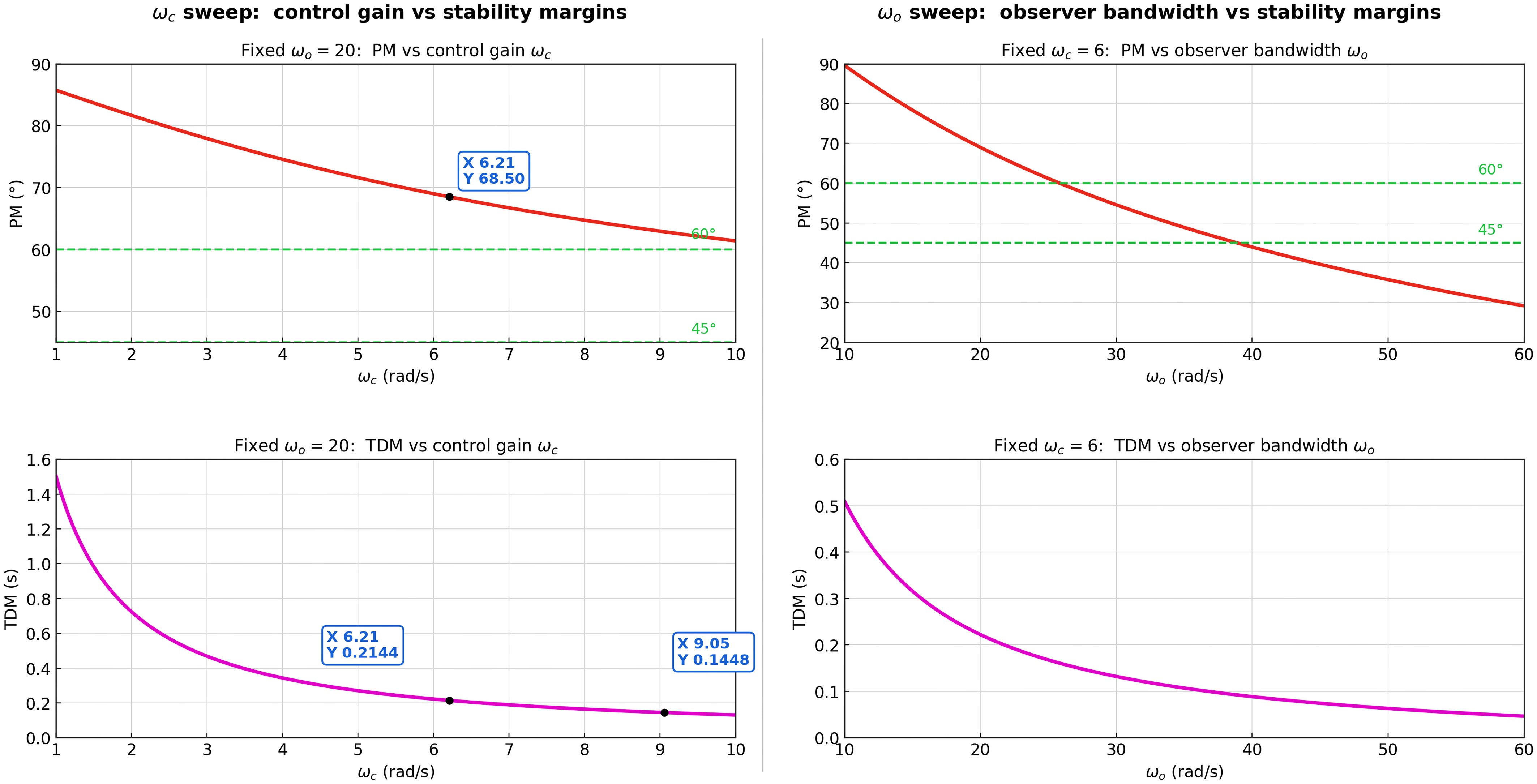
Figure 6.
Simulation verification of stability margins. Left: control-gain sweep ($ \omega_c $) at fixed $ \omega_o $ = 20 rad/s. Right: observer-bandwidth sweep ($ \omega_o $) at fixed $ \omega_c $ = 6 rad/s. Dashed lines mark the 45° and 60° PM references.
Table 3 summarizes the margins read from these sweeps at the design-relevant operating points. The adopted gains
$ k_q $ $ k_p $ $ \omega_c $ $ \omega_c $ $ \omega_o $ $ k_{\theta} $ $ k_{\phi} $ Table 3. Stability margins at the design operating points (from the sweeps of Fig. 6).
Operating point GM (dB)* PM TDM (ms) Level 1/margin spec $ \omega_c $ = 6, $ \omega_o $ = 20 ≥ 6 68.5° 214 Adopted design point—met $ \omega_o $ ≈ 40 rad/s – = 45° ≈ 90 Observer-bandwidth ceiling $ \omega_o $ > 40 rad/s – < 45° < 90 Over-fast observer: margins eroded * The gain margin (GM) at the adopted design point is specified by design to be ≥ 6 dB. These results give three porting rules for the present platform. First, the recommended operating band is
$ \omega_c $ $ \omega_o $ $ \omega_c $ Key protection and control logic during launch
Protection logic for acceleration saturation during the launch process
-
The acceleration during ejection is shown in Fig. 7. At the moment of ejection, the acceleration reaches 175 m/s2, which exceeds the IMU's maximum range of 160 m/s2. This data saturation results in inaccurate acceleration readings, leading to errors in velocity and position calculations, and consequently causing significant drift and error accumulation in the navigation solution. To address this issue, we disregard the IMU's acceleration data before launch and instead use the theoretically calculated launch velocity.
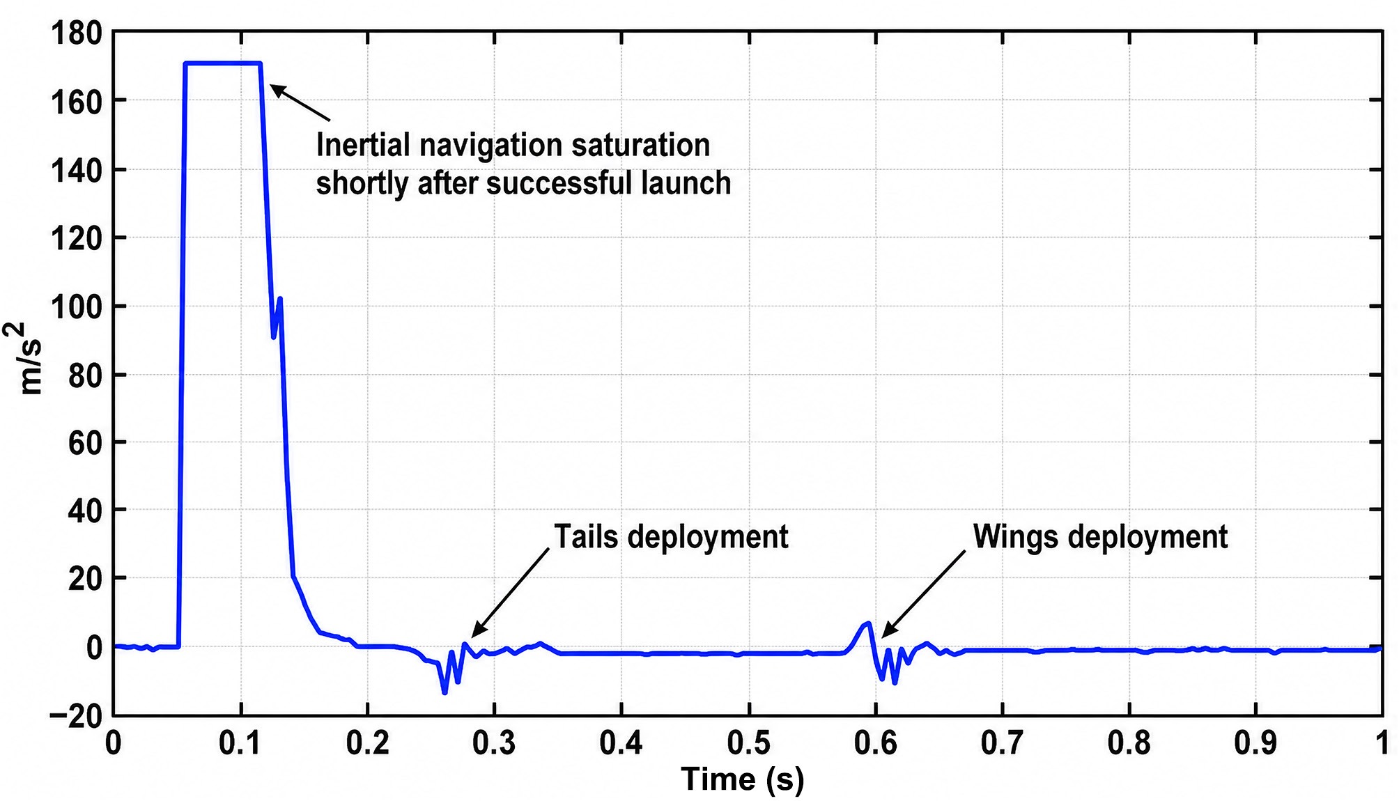
Figure 7.
The evolution of acceleration vs time throughout the whole launch process.
Identification of V-tail/wing deployment window based on acceleration fluctuation (T2, T3)
-
Through the analysis of the acceleration data of the ejection tests, it is found that there will be two acceleration fluctuations during the launch process, which are caused by the expansion of the V-tail and the wing. Therefore, the exact deployment windows of the V-tail and the wing, namely T2 and T3, can be obtained. Based on the V-tail and wing deployment time, the elevator and aileron participation closed-loop stabilization control time can be determined.
Segmented throttle control strategy (suppression of roll peak upon motor startup)
-
To eliminate the sharp roll torque peak induced by a sudden full-speed start of the propulsion motor, a segmented throttle scheduling scheme is designed in this subsection. The motor output power is increased gradually in multiple staged increments rather than by a one-step maximum command. The step size and holding time of each throttle segment are matched with the structural unfolding sequence. This gentle power-up mode weakens the instantaneous asymmetric rolling moment, restrains the peak roll angular rate, and alleviates the regulation burden of the attitude control loop.
Simulation results of launch process stability
-
According to the previous launch data, it can be known:
The first disturbance is introduced 0.1 s after the ejection; the second disturbance is introduced 0.5 s after a successful launch; and the third disturbance is introduced 1.5 s after a successful launch. As shown in Fig. 8, the orange curve represents the roll angular rate, and the blue curve represents the pitch angular rate. It can be concluded that, after wing deployment, all actuators can normally participate in control, and the disturbances exerted at T2 (V-tail deployment) and T3 (wing deployment) are quickly suppressed. Two seconds after the propulsion motor starts, the vehicle's angular rates converge to 0 rad/s, and the attitude is stabilized, demonstrating that the ESO-based control method effectively enhances launch-phase stability.
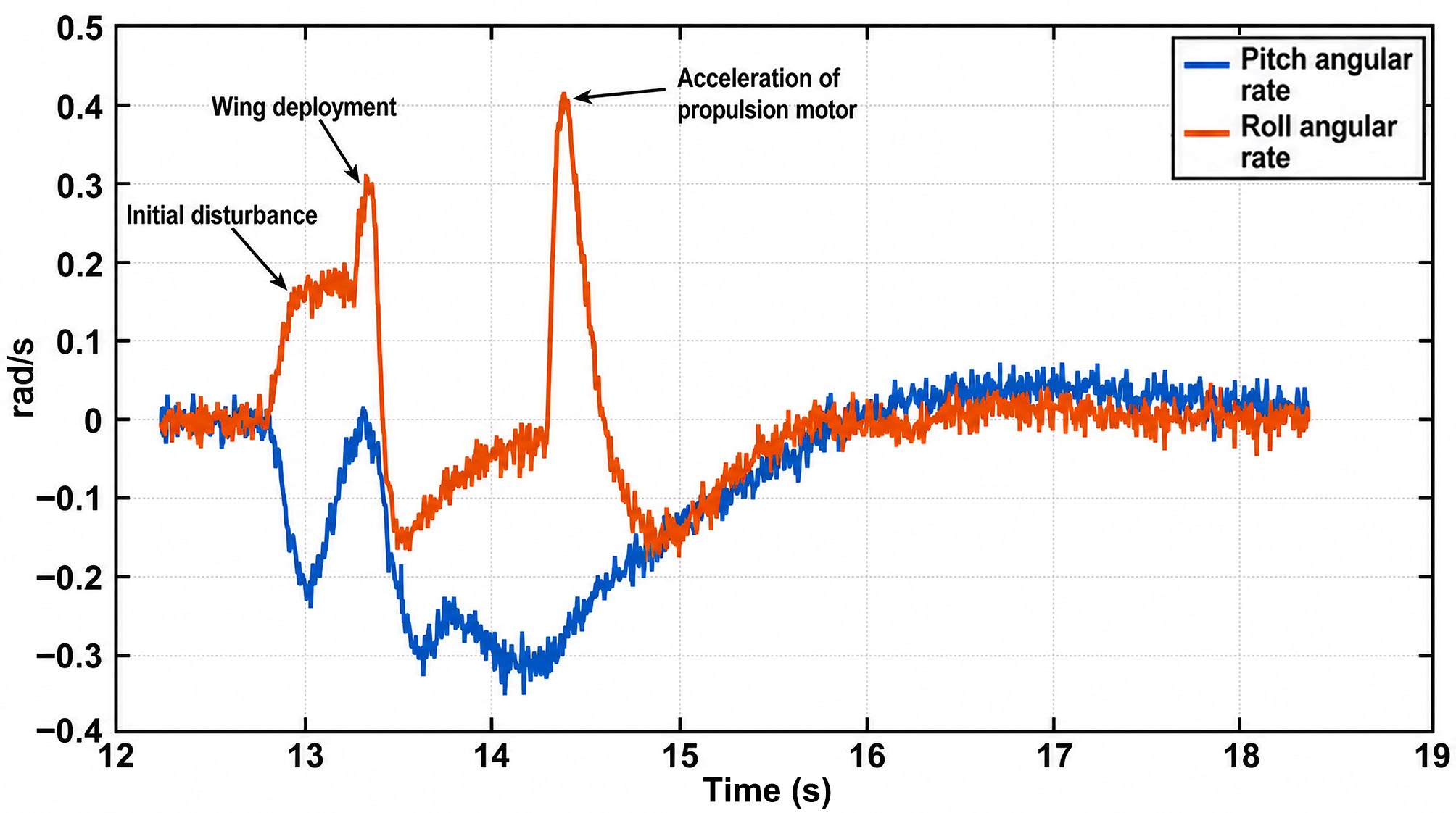
Figure 8.
Time histories of the roll angular rate without adopting segmental throttle control strategy.
But at T4, the full rate of the propulsion motor leads to a relatively large roll angular rate peak. To reduce this undesired peak, we introduce a practical segmental throttle control strategy. The throttle whole acceleration process is divided into two stages:
• Increase the throttle from 0% to 80%, while maintaining the throttle steady at 80% for 0.5 s.
• Increase the throttle from 80% to 100%.
The time histories for the roll and pitch angular rate adopting the segmental throttle control strategy are shown in Fig. 9. It can be concluded that the peak value of roll angular rate decreases from 0.42 rad/s initially to 0.26 rad/s currently, which makes the vehicle attitude more stable and achieves the desired goal.
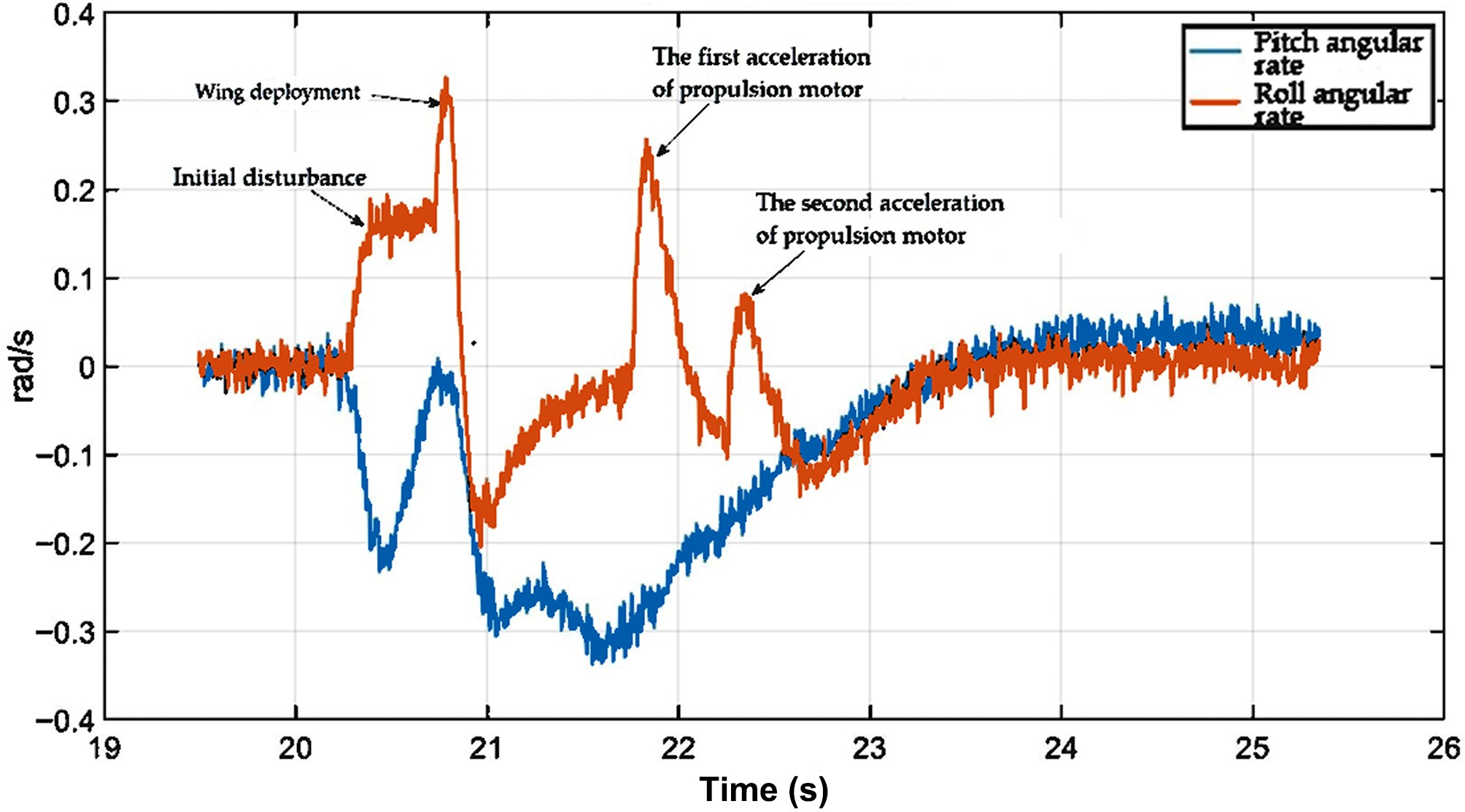
Figure 9.
Time histories of the roll angular rate adopting the segmental throttle control strategy.
Robustness verification: Monte Carlo simulation
Parameter perturbation settings (inertia, control coefficient, aerodynamic coefficient, thrust)
-
To better verify the robustness and tracking performance under model parameter perturbations, Monte Carlo simulations are conducted. The related uncertainties are shown in Table 4.
Table 4. Parameter perturbations in Monte Carlo simulations.
Parameter Uncertainty (%) Inertial parameters ± 30 Control coefficients ± 20 Aerodynamic coefficients ± 40 Engine thrust ± 10 The perturbation ranges in Table 4 are determined from the way the corresponding nominal parameters are obtained, together with worst-case engineering estimates. The inertial parameters are extracted from the three-dimensional Computer-Aided Design (CAD) model in CATIA, and a relatively wide band of ± 30% is adopted to bound the residual error between the CAD-based mass distribution and the as-built vehicle. The control and aerodynamic effectiveness coefficients are computed by CFD, in which the slipstream effect is not considered; a band of ± 20% for the control coefficients and ± 40% for the aerodynamic coefficients is therefore used to cover both the CFD modelling error and the neglected slipstream contribution. The engine thrust is measured by a ground static-thrust test, and a tighter band of ± 10% is assigned in accordance with the repeatability of the measurement and the expected installation losses.
Monte Carlo results: statistics of pitch/roll channels
-
Latin hypercube sampling[20] is utilized in the Monte Carlo simulations to achieve small-sample convergence. In addition, 100 Monte Carlo tests are shown in Figs 10 and 11.
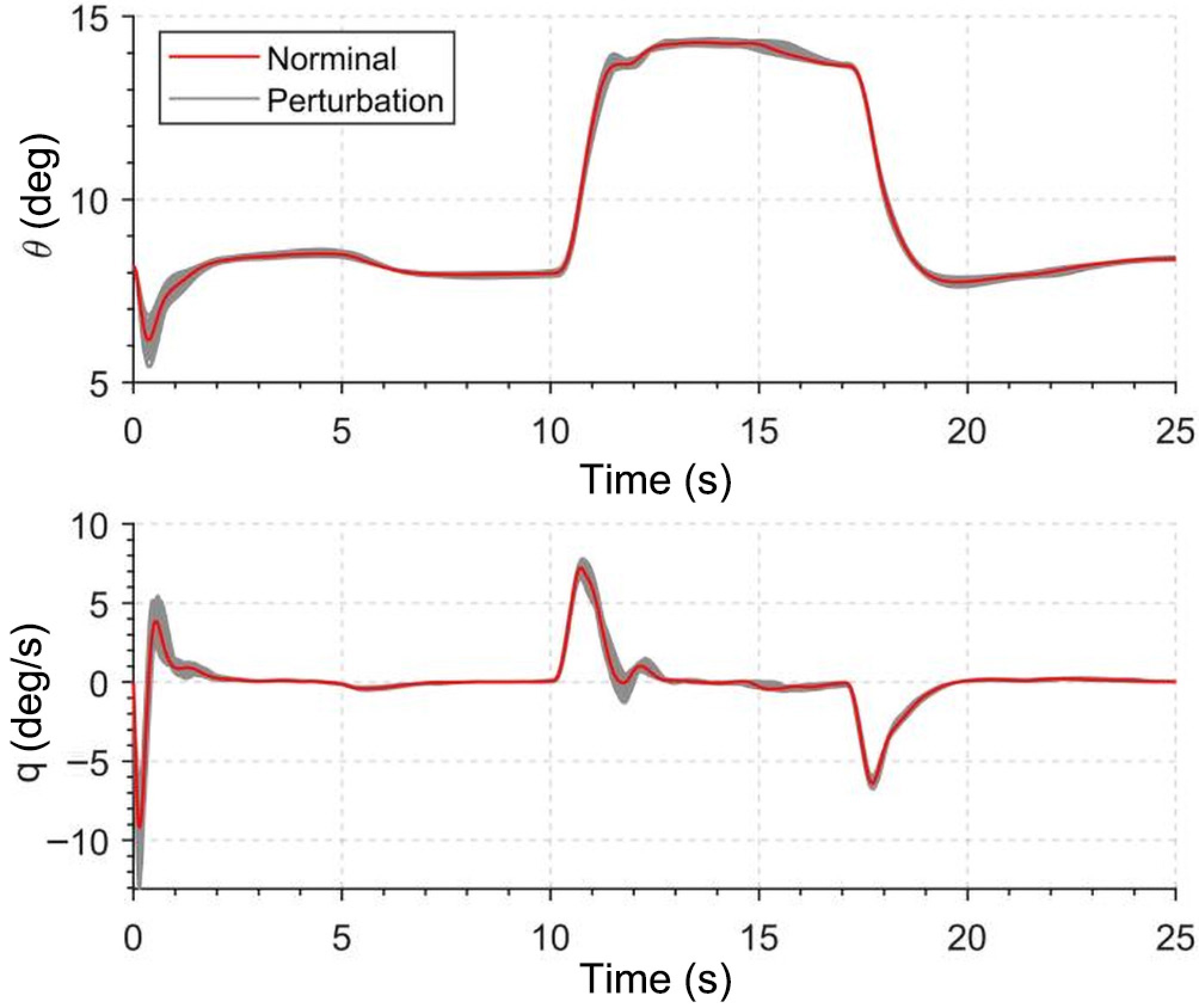
Figure 10.
Results of Monte Carlo simulations of the ESO-based pitch control.
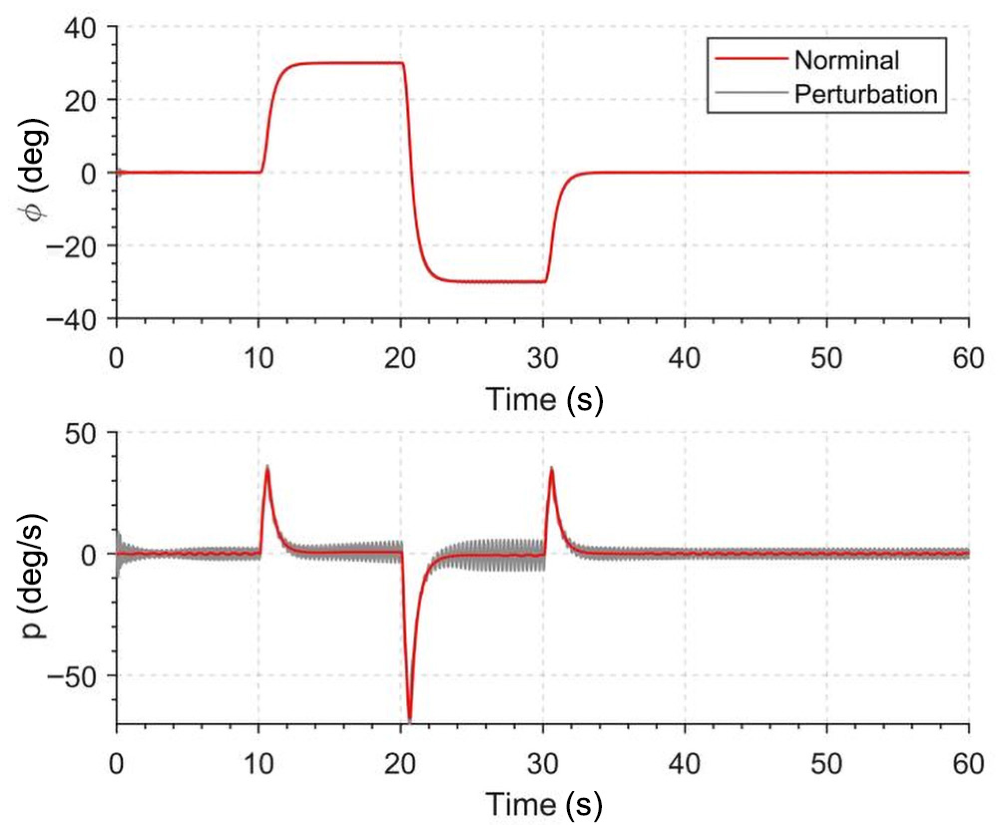
Figure 11.
Results of Monte Carlo simulations of the ESO-based roll control.
After completing batches of random sampling simulations, this subsection conducts statistical sorting and quantitative analysis on massive operating data. Key evaluation metrics covering maximum attitude deviation, peak angular rate, actuator saturation frequency, and steady-state tracking error are counted for all sampling cases. The overall distribution range and failure-free proportion of each index are summarized. It can be seen that even with simultaneous deviation of inertia, aerodynamic coefficients, control gains, and thrust within the preset perturbation bounds, the combined scheme of deployment window identification, segmented throttle, and cascaded ADRC still restrains attitude fluctuation within safe allowable limits. The statistical outcomes fully verify that the designed launch control system possesses strong parameter robustness and environmental adaptability.
Criteria for the successful launch process
-
We conclude four criteria for the successful launch process:
• The pitch angular rate should be limited to ± 0.5 rad/s before the motor is activated.
• After the wings are deployed, the roll angular rate should converge to ± 0.1 rad/s within 0.5 s.
• After the throttle reaches 100%, the roll angular rate should converge to ± 0.05 rad/s within 1.5 s.
• After the throttle reaches 100%, the pitch angular rate should converge to ± 0.05 rad/s within 2 s.
-
To fully verify the superiority of the proposed cascaded ADRC controller, comparative tests are performed against two typical control strategies, namely conventional PID and nonlinear model predictive control (NMPC). All controllers are configured with the same control bandwidth and actuator constraints. Typical launch disturbances, including wing deployment impact, launcher friction-induced rotation, and motor reverse torque, are applied to the system. To evaluate the performance of the proposed ADRC controller, the following tracking performance index is considered:
$ \begin{aligned} {\rm{MSE}}=\dfrac{1}{T}\int_{0}^{T}\bigl(\theta_c(t)-\theta(t)\bigr)^2\,dt \end{aligned}. $ (29) In Table 5, we tabulate the performance index for each case. The results show that the proposed ADRC achieves the lowest tracking error.
Table 5. Tracking errors of different control methods.
Method Value ADRC 1.5 PID 3.9 NMPC 2.4 To ensure a fair comparison, the PID controller is not tuned heuristically: its gains are obtained with the MATLAB PID Tuner, in which the target closed-loop bandwidth is fixed to the same value as that of the proposed ADRC, and the final parameters are then determined by the built-in optimization algorithm to balance tracking accuracy and stability margins. The NMPC controller is likewise configured with the same control bandwidth and actuator constraints.
Real-world validation
Flight test hardware system and test environment conditions
-
The flight test was conducted on the gun-launched variable-geometry UAV platform shown in the figure above. The tests were performed in an open outdoor field under normal daytime atmospheric conditions, with light-to-moderate ambient wind. During the trials, the vehicle was subjected to realistic launch disturbances, including launcher-induced rotation at ejection, the impact of wing and tail deployment, and the reaction torque of motor start-up, as well as atmospheric gusts and the run-to-run inconsistency inherent to the launch process. These conditions confirm that the data analyzed below were obtained in a representative real flight environment rather than under idealized settings.
We implemented the flight-control system using a MATLAB/Simulink design flow with Embedded Coder to generate C code for direct deployment. For hardware configuration, the Hardware-in-the-Loop (HIL) simulations were conducted using the autopilot (CPU: STM32F765VGT6,216 MHz) and the simulator (CPU: ARM Cortex-A53, 1.2 GHz). The controllers run at 400 Hz, and the guidance loop runs at 20 Hz.
Flight data analysis
-
Prior to the real-world flight, an extensive series of Monte Carlo simulations was conducted. Throughout the mission scenario, the bandwidth parameters of the extended state observer (ESO) remained fixed, except for
$ b_q $ 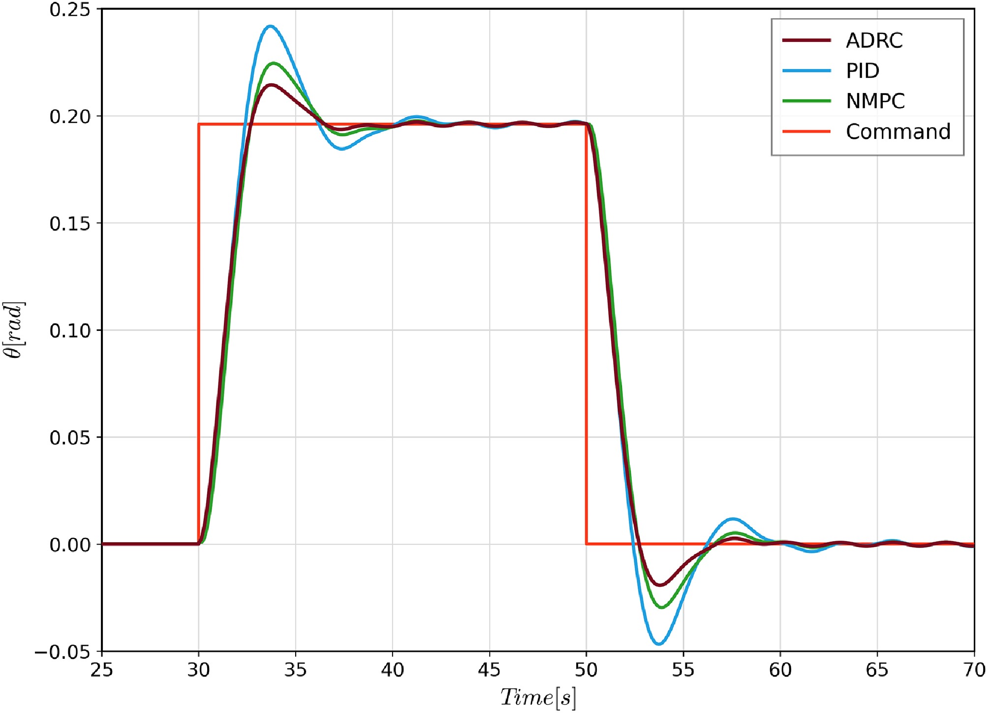
Figure 12.
The pitch angle tracking performance comparison among ADRC, PID, and NMPC.
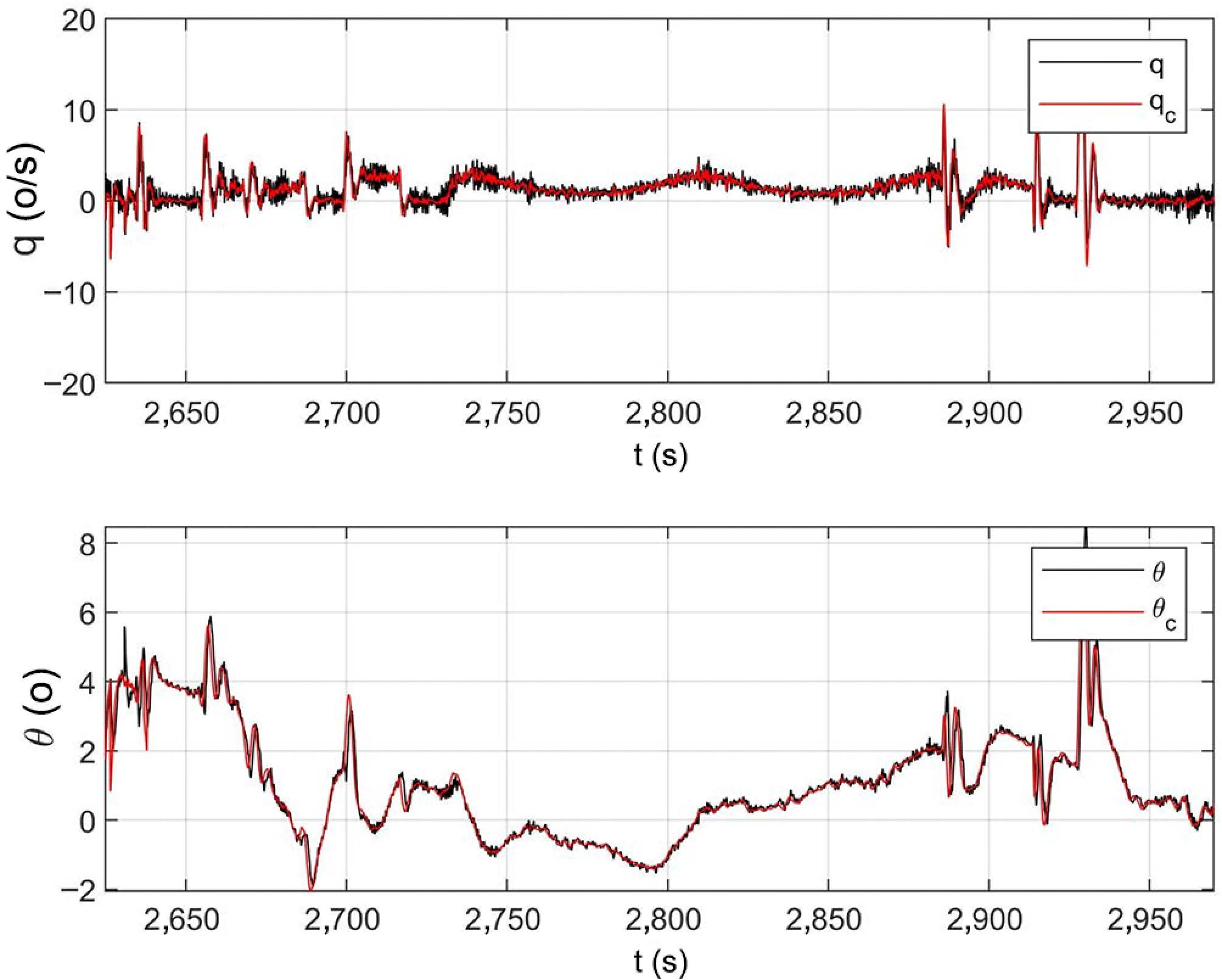
Figure 13.
Time histories of the pitch channel.
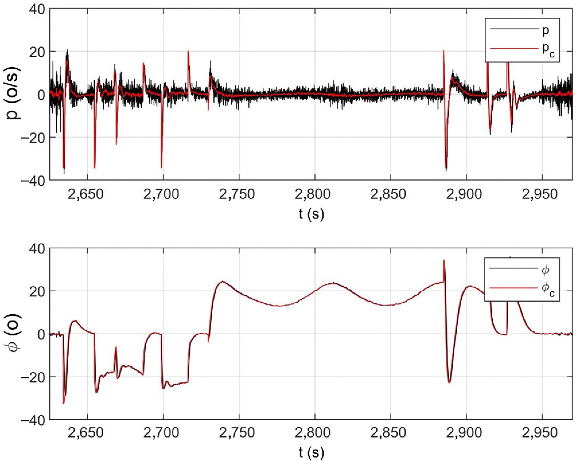
Figure 14.
Time histories of the roll channel.
The actual flight data plotted in Figs 13 and 14 cover the time window of approximately t = 2,650 − 2,950 s, which corresponds to the steady cruise phase after launch rather than the ejection process. These long-duration flight curves are supplemented to further validate the long-term steady-state tracking capability of the cascaded ADRC controller. Apart from anti-disturbance performance during launch and wing deployment, the controller can maintain high-precision stable attitude regulation under continuous steady flight conditions, verifying the full-envelope applicability of the proposed control strategy throughout the whole flight mission.
Limitations
-
Several limitations of the present study should be noted. First, the control design and validation focus on the launch phase and the subsequent cruise condition of a specific gun-launched variable-geometry UAV; the conclusions therefore apply to this configuration and flight envelope, and extension to other vehicles or to the full mission profile would require further verification. In addition, the aerodynamic and control-effectiveness coefficients are obtained from CFD without accounting for the propeller slipstream, and the parameter perturbation bounds are estimated from the data sources and worst-case engineering judgment rather than from a large statistical sample, so the robustness results should be read as representative rather than exhaustive. Finally, the real-world validation is based on a limited number of flight tests covering a steady cruise window rather than a large campaign spanning the complete launch-to-recovery envelope under diverse atmospheric conditions. Addressing these aspects, including slipstream-coupled aerodynamics and more extensive flight testing, constitutes our future work.
-
This paper investigated a disturbance rejection control strategy for a variable-geometry, gun-launched UAV. To design a more accurate control law, modal analysis of the aircraft deployment configuration under a nominal mission scenario was first performed. Subsequently, a dedicated control strategy for the launch process was proposed, and a cascaded active disturbance rejection control (ADRC) attitude control system was developed. In addition, a timescale-separation tuning principle was introduced to facilitate the adjustment of the control gains. Monte Carlo simulations and real-world flight validations verified the effectiveness of the proposed launch control strategy and control system. Both simulation and flight results demonstrated improved control stability and robustness: the maximum and mean roll angular rates were reduced by 26% and 33%, respectively, and the maximum and mean pitch angular rates were reduced by 13% and 21%, respectively.
-
The authors confirm their contributions to the paper as follows: conceptualization: Wang Z, Xu C; methodology, formal analysis: Wang Z, Liu G; software, writing – original draft preparation: Wang Z; validation, investigation: Wang Z, Liu G, Yi J; resources: Cui C, Liu Y, Xu C; data curation: Wang Z, Cui C; writing – review and editing: Liu G, Cui C, Yi J, Liu Y, Xu C; visualization: Wang Z, Yi J; supervision, funding acquisition: Xu C; project administration: Liu Y, Xu C. All authors reviewed the results and approved the final version of the manuscript.
-
The flight test data and simulation datasets generated and analyzed during this study are available from the corresponding author upon reasonable request. The data include raw IMU measurements, attitude angles, angular rates, and control surface deflections recorded during the launch phase. Due to the sensitive nature of the UAV platform parameters and proprietary constraints of the collaborative research project, the complete aerodynamic model and embedded control code are not publicly available. Requests for access to the data should be directed to the corresponding author (Chao Xu) and will be evaluated on a case-by-case basis.
-
The authors declare that they have no conflict of interest. This research was supported by the Natural Science Foundation of Zhejiang Province. The funding source had no involvement in the study design, data collection, analysis, decision to publish, or preparation of the manuscript. The authors have no financial or personal relationships with other people or organizations that could inappropriately influence or bias this work.
- Copyright: © 2026 by the author(s). Published by Maximum Academic Press, Fayetteville, GA. This article is an open access article distributed under Creative Commons Attribution License (CC BY 4.0), visit https://creativecommons.org/licenses/by/4.0/.
-
About this article
Cite this article
Wang Z, Liu G, Cui C, Yi J, Liu Y, et al. 2026. Launch phase robustification of a gun-launched unmanned aerial vehicle for rapid reaction missions. International Journal of Micro Air Vehicles 18: e022 doi: 10.48130/mav-0026-0023 

Launch phase robustification of a gun-launched unmanned aerial vehicle for rapid reaction missions
- Received: 02 April 2026
- Revised: 15 July 2026
- Accepted: 11 August 2026
- Published online: 30 October 2026
Abstract: Gun-launched unmanned aerial vehicles (GL-UAVs) are novel aircraft designed for rapid-response tasks such as emergency rescue and forest and wildfire patrols. During launch, unavoidable operational factors lead to variable-geometry disturbances, intense launch overload, and motor counter-torque. Structural deformation arising from wing and empennage deployment reshapes the UAV's outline and aerodynamic characteristics, altering lift, drag, and control torque, and consequently causing response lag or overshoot in the control system. To address these uncertain dynamics, this paper presents a disturbance-rejection control scheme tailored for the launch phase: an angular-rate tracking active disturbance rejection control (ADRC) approach based on the extended state observer (ESO), which realizes real-time estimation and compensation of lumped disturbances and model uncertainties. Moreover, segmented throttle control is deployed to curb peak roll angular velocity induced by counter-torque when motors start up. Monte Carlo simulations and actual flight tests confirm the effectiveness of the proposed launch control algorithm and manual stability augmentation strategy.