A slower-than-needed scale-up of renewable energy might reduce the incentive for mitigation

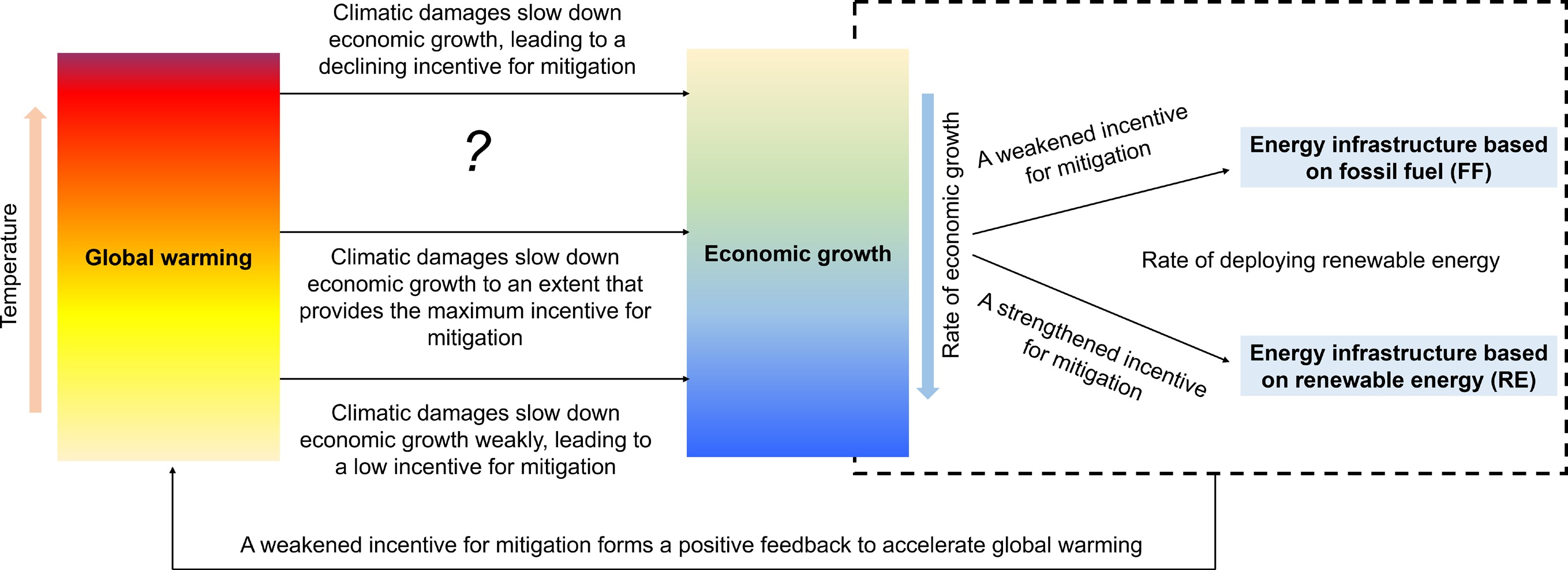
Earth's surface air temperature has approached 1.5 °C warming relative to pre-industrial levels since 2024, with a rising likelihood of surpassing 2 °C by the end of this century^[1]. Rapid climate change is threatening the habitability of our planet by increasing the risks of extreme weather, glacial retreat, sea level rise, collapse of ocean and terrestrial ecosystems, zoonotic diseases, and compound stresses^[2]. Given the geophysical and technological constraints on nature-based solutions or ecosystem-based approaches, reducing the risk of catastrophic climate change requires an accelerated transition from fossil fuels to renewable energy^[3,4]. However, global CO₂ emissions have continued to rise following the coronavirus disease (COVID-19) pandemic^[5], mainly through stimulated consumption^[6], carbon-intensive infrastructure lock-in^[7], rapidly growing energy demand^[8], and geophysical, technological, and socioeconomic barriers to renewable energy's deployment^[9,10]. Achieving a high share of renewable energy is hindered by profit protection in the existing fossil fuel industries^[11], current economic recovery policies^[6], socioeconomic inertia in transitioning the workforce and investment from fossil fuels to renewable energy^[12], and financial disruptions from phasing out fossil fuels^[13]. Some countries have even rolled back mitigation policies becasue of their stranded fossil fuel assets, posing an emergent threat to coherence in global mitigation^[14]. As a result, the world is likely on track toward 3 °C warming under current policies or Nationally Determined Contributions (NDCs), indicating a serious deviation from the economically optimal pathway compatible with a global warming objective of 2 °C or less^[15−17]. The hesitant actions in mitigation are consistent with a tendency to take a "wait-and-see" approach^[18,19], which prefers to defer mitigation because of both the high short-term mitigation costs^{[9,10,20−22]} and uncertain long-term mitigation outcomes^[23−34]. The hypothesis of this strategy is that if mitigation is delayed, the incentive for mitigation would increase as climatic damages increase as a result of the continuous rise in temperature^[16,17,35]. However, some climatic damages might rise initially and then decline rapidly after crossing a tipping point, leading to a diminishing incentive for mitigation^[36−39]. This study therefore tests the hypothesis that delaying strong mitigation to phase out fossil fuels could produce a self-reinforcing disincentive, undermining global mitigation efforts (see a schematic illustration of this hypothesis in Fig. 1).

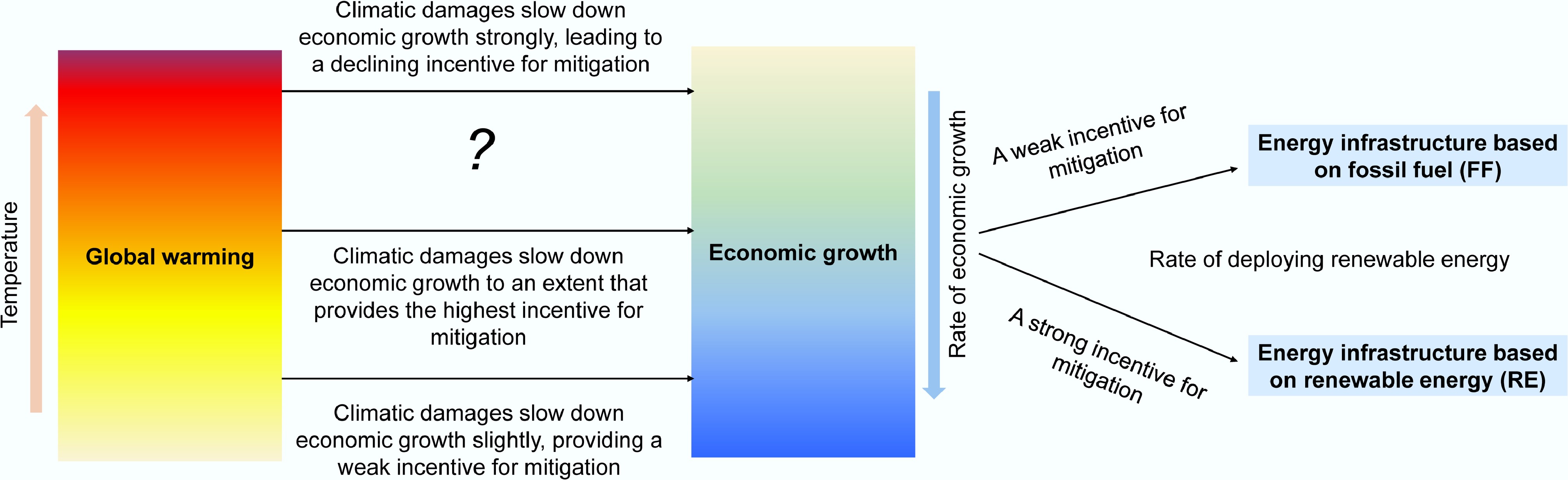
Figure 1. 

Schematic illustration of the hypothesis tested in this study. The study examines whether delaying the initiation of strong incentives for mitigation and to phase out fossil fuels could produce a self-reinforcing disincentive, thereby undermining global mitigation efforts.

To address the question of when and how to tackle climate change, integrated assessment models (IAMs) have been developed to provide policy-relevant insights into the economically optimal mitigation pathways (e.g., refs^{[2,6,12,16,21,23,28−37,39−42]}). Increasing evidence highlights the existence of barriers to deep decarbonization when achieving a high share of renewable energy^[20−22], limited potential for reducing renewable energy prices on the basis of the empirically grounded effects of technological advances^[9,10,43], and the tremendous economic damage caused by climate change in the past decade^[27−29]. These factors necessitate a re-examination of the optimal strategy for tackling climate change within the IAMs^[15,17−23]. For example, the costs of mitigation to achieve net-zero CO₂ emissions in all sectors through the deployment of a set of "backstop" technologies are postulated to decrease from USD${\$} $550 to USD${\$} $120 per tonne of CO₂ emissions (tCO₂) between 2010 and 2100 (e.g., refs.^[16,35]). Meanwhile, damage caused by climate change was projected to grow nonlinearly from 0.1%−0.5% to 1%−2% of gross domestic product (GDP) as global warming rises from 1 to 2 °C (e.g., refs.^[16,17]) and to reach up to 50% of GDP as global warming reaches 6 °C (e.g., refs.^[23]). As a result, the time of initiating strong mitigation actions to phase out fossil fuels could be deferred to the years after 2100 in many IAM scenarios^[2].

To examine the hypothesis in this study, I account for socioeconomic feedback resulting from delayed mitigation by modifying an IAM^[44] that optimizes intertemporal decisions on consumption and labor allocations and investments under welfare maximization (see the Methods section). The social cost of carbon (SCC), as an indicator of the incentive for mitigation, is estimated as the total discounted damages in the future that are attributed to an increase in tCO₂ emissions in a given year^[35,41].

I compare SCC under a constant pure rate of time preference (PRTP) (ρ = 0.5%)^[42] across various scenarios, where strong mitigation is initiated by reducing the PRTP from 5% to 0.5% starting in a specific year (e.g., 2030, 2040, … 2075) to protect future wellbeing. This approach illustrates how the SCC responds to global warming when mitigation is delayed to a future year. To evaluate uncertainties in the SCC and global warming, I run 10,000 Monte Carlo simulations by randomly varying the key parameters in the IAM (see Supplementary Tables S1 and S2 for a list of equations and key parameters). Lastly, I derive the relationship between the renewable energy share and climatic damages when mitigation begins in different years, enabling the identification of an early-warning signal of the declining incentive for mitigation.

Continuous efforts have been made to improve IAMs (e.g., refs.^{[2,6,12,16,21,23,28−37,39−42]}) by integrating knowledge from fields including climate change, economic growth, energy transitions, and other aspects of human and natural societies to holistically understand the interactions between human activities and natural systems when addressing complex issues like climate change and sustainable development. A standard IAM couples an energy−economy model (i.e., simulating how energy is produced, distributed, and consumed, plus how this relates to economic growth and social development) with a climate model (i.e., simulating the physical processes of the climate system, including how greenhouse gas emissions interact with temperature, precipitation, and other climate variables), and potentially a socioeconomic model (i.e., simulating how human populations, economies, and societies respond to climate change) to identify optimal strategies of climate mitigation^{[2,6,12,16,21,23,28−37,39−42]}. In this study, the IAM^[44] is modified by accounting for the energy−economy−climate interactions based on the evidence for economic barriers to achieving a high renewable energy share^[20−22], limited potential for reducing renewable energy costs^[9,10,43], and the observed economic damage caused by climate change^[27−29] (see Supplementary Table S1 for a list of equations with their interpretation and methods of calibration; see Supplementary Table S2 for a list of parameters with their values and methods of parameterization).

I optimize the intertemporal decisions on consumption behaviors (C_t) and the allocation of investment (I_t) and labor (L_t) among sectors producing fossil fuel, renewable energy, and nonenergy products. The GDP is produced by taking energy (E_t) and nonenergy products (B_t) as inputs in a constant elasticity of substitution (CES) function^[44] (Eq. [1]). I consider that the useful energy product (E_t) is produced by aggregating fossil fuels (F_t) and renewable energy (G_t) in a CES function. Let i_s,t denote the rate of saving (the ratio of investment to output); i_e,t and j_e,t denote the fraction of total labor and investment allocated to the energy sector, respectively; i_g,t and j_g,t denote the fraction of labor and investment in the energy sector allocated to produce renewable energy, respectively; L_d,t, L_g,t, and L_b,t denote labor producing fossil fuels, renewable energy, and nonenergy products, respectively; K_d,t, K_g,t, and K_b,t denote capital producing fossil fuels, renewable energy, and nonenergy products, respectively; and d_t denotes the damage caused by climate change as a percentage of GDP, expressed as a function of global warming (ΔT_t). I then optimize the intertemporal decisions on consumption and the allocation of labor and investment to maximize the welfare (W), defined as the discounted sum of the population-weighted utility of per capita consumption:

where, t is the time, ρ is the PRTP, δ is the elasticity of consumption (1.5), γ is the elasticity of output to capital (0.3), σ_Y is the constant elasticity of substitution between energy and nonenergy products^[45], σ_E is the constant elasticity of substitution between fossil fuel and renewable energy, η_e,t is the energy use efficiency, β_b,t is the efficiency of producing nonenergy products, and β_d,t and β_g,t are the efficiency of producing fossil fuels and renewable energy. Moreover, λ_w is the constant coefficient calibrated to reach a level of damage (0.1%−0.5%) when global warming is 1 °C^[46], d_c is the climatic damage as a percentage of GDP (25%−75%) after crossing catastrophic tipping points in the climate system^[36], k is a constant (6 ± 1), T₅₀ is the threshold of global warming leading to 50% of climatic damage after crossing catastrophic tipping points (T₅₀ = 2 ± 0.5 °C), ΔT_t is the global warming in a year (t), ΔT₂₀₂₀ is global warming in 2020 (1.1 ± 0.1°C)^[47], τ_R is the lag time of the response in global warming to CO₂ emissions (10 ± 10 years)^[48], τ_L is the lifetime of CO₂ in the atmosphere (400 ± 200 years)^[47], φ is a constant calibrated by the response of global warming to global cumulative CO₂ emissions, ϱ_F is the ratio of global CO₂ emissions to the global consumption of fossil fuels (depending on the composition of fossil fuels, which is calibrated by historical data)^[44], and θ is the rate of capital depreciation (0.1)^[46]. I calibrate the response of global warming to cumulative CO₂ emissions (φ) on the basis of the observed global warming and historical CO₂ emissions^[2] with a lag time (τ_R) of 10 ± 10 years^[48] and a lifetime (τ_L) of 400 ± 200 years for CO₂ in the atmosphere^[47].

I adopt a range for the rate of growth in productivity (k_p = 1 ± 0.5% per year) based on the rate of economic growth in the shared socioeconomic pathway (SSP) scenarios^[49]. I adopt a range for the rate of growth in energy-use efficiency (k_u = 1%−5% per year) to account for the impact of energy-saving technological advances^[44]. I apply Wright's law to predict the rate of growth in the efficiency of producing renewable energy (β_g,t), based on the empirically grounded learning rate (L_R)^[43]. Therefore, the growth in efficiency is predicted to be^[43,44]:

The price of renewable energy is derived as a first-order derivative of the output to renewable energy^[44]:

Calculation of the SCC

The social cost of carbon (SCC_t) is calculated as the discounted economic damage caused by an increase in tCO₂ emissions at present^[35,41]:

where, t is the year adding CO₂ emissions, W is welfare, C_t is the annual consumption of economic output, L_t is the total population, F_t is the annual consumption of fossil fuels, ϱ_F is the ratio of global CO₂ emissions to the global consumption of fossil fuels, and δ is the elasticity of consumption (1.5). I estimate the SCC under a constant PRTP (ρ = 0.5%)^[42] for different scenarios, where strong mitigation is initiated in a specific year (e.g., 2030, 2040, …, and 2075) by reducing the PRTP from 5% to 0.5% to introduce a strong incentive for mitigation to protect wellbeing in the future. I calibrate PRTP in 2020 (ρ = 5%) on the basis of the current share of renewable energy in the global energy supply (20%)^[50].

I optimize the intertemporal decisions on consumption and the allocation of labor and investment to reduce the climatic damage in the future by controlling the rate of energy transition from fossil fuels to renewable energy under welfare maximization (Fig. 2a). I employ a CES function^[51] to predict the production of energy and GDP (Fig. 2b). This function is suggested to perform better than the Cobb-Douglas function^[52] in predicting the historical rates of change in the efficiency of energy consumption, energy use, and energy production, as well as economic output^[44] (Supplementary File 1). I adopt the elasticity of substitution between energy and nonenergy inputs (σ_Y = 0.5 ± 0.4 as the 95% confidence interval hereafter), which was calibrated using observed changes in energy consumption in response to a change in the price of energy across 30 sectors in the United States^[53]. At the same time, I consider a wide range of the elasticity of substitution between fossil fuels and renewable energy (σ_E = 1−4) to represent the intermittent nature of renewable energy^[9] and the spatiotemporal mismatch between the production of renewable energy and the power demand^[54]. I apply a range of 15% ± 10% for the learning rate (L_R), which was calibrated on the basis of historical rates of decline in renewable energy prices^[43]. Considering the effect of technological advances in the model, I show that mitigation costs may increase more rapidly as CO₂ emissions are further reduced and deeper decarbonization is achieved (Fig. 2c, d). For example, GDP is projected to decrease by 7%−8% (σ_E = 1) or 5%−6% (σ_E = 3) when the supply of fossil fuel is reduced by 50%. In contrast, GDP is projected to decrease by 34%−51% (σ_E = 1) or 21%−31% (σ_E = 3) when the supply of fossil fuel is reduced by 90%. This can be explained by the fact that the geophysical and technological constraints associated with deploying renewable energy could be stringent with a high share of renewable energy within total energy^[20−22,44].

Figure 2. 

Economics of climate mitigation. (a) Structure of the integrated assessment model used in this study. (b) Trade-offs between two quantities (E and B) when producing the same output (Y) in the CES function. The variable σ denotes the elasticity of substitution between E and B. The dashed line denotes the marginal increase in E that is needed to offset the effect of reducing B when producing the same output. (c) Dependence of the costs of mitigation as a percentage of GDP on the elasticity of substitution between energy and nonenergy inputs (σ_Y) and the elasticity of substitution between fossil fuel and renewable energy (σ_E). (d) The fraction of decrease in the price of renewable energy resulting from technological advances, based on the learning rate (L_R). (e) Dependence of climatic damage as a percentage of GDP on global warming for different values of the coefficients T₅₀, d_c, and k within the damage function^[23]. For comparison, the black line denotes the damage curve in the Dynamic Integrated Model of Climate and the Economy (DICE) model^[46], the box denotes a bottom-up estimate as a part of CO-designing the Assessment of Climate Cange (COACCH) Project 27, the circle denotes a top-down estimate^[28,29], and the triangle denotes an estimate from a statistical model^[30].

I employ an empirical function from the literature^[23] to predict the economic damage caused by climate change as a percentage of GDP. In this function, λ_w is a quadratic coefficient calibrated on the basis of the observed damage (i.e., 0.1%−0.4% of GDP) when global warming is 1 °C^[46], d_c denotes the climatic damage (i.e., 25%−75% of GDP) caused by crossing catastrophic tipping points in the climate system^[36], T₅₀ denotes the threshold of global warming leading to 50% of the climatic damage caused by crossing catastrophic tipping points, and k is a constant (6 ± 1). I select a range of T₅₀ (i.e., 1.5−2.5 °C) to align with temperature targets in the Paris Agreement^[2]. Using this damage function in the model, I predict a larger climatic damage (i.e., 20%−50% of GDP) at 2 °C warming than the Dynamic Integrated Model of Climate and the Economy (DICE) model (i.e., ~1% of GDP)^[46], whereas my estimate is closer to a bottom-up estimate (i.e., 5%−15% of GDP)^[27], a top-down estimate (i.e., 25%−35% of GDP)^[28,29], and the empirically grounded estimate using a statistical model (i.e., 15%−40% of GDP)^[30] (Fig. 2e).

Pathway of energy transition

I next explore the pathway of energy transition by characterizing how consumption behavior and the allocation of investment and labor respond to the initiation of mitigation by introducing an abrupt reduction in the PRTP from 5% to 0.5% (Fig. 3). This leads to an abrupt increase in the saving rate and an accelerated transition from fossil fuels to renewable energy, while the consumption of fossil fuels depends on the total energy demand. There is an increasing energy demand driven by economic growth caused by improvements in the efficiencies of producing renewable energy and nonenergy products. However, technological advances in energy-use efficiency could reduce the energy demand, even when rebound effects are considered^[44,53] (Supplementary Fig. S1).

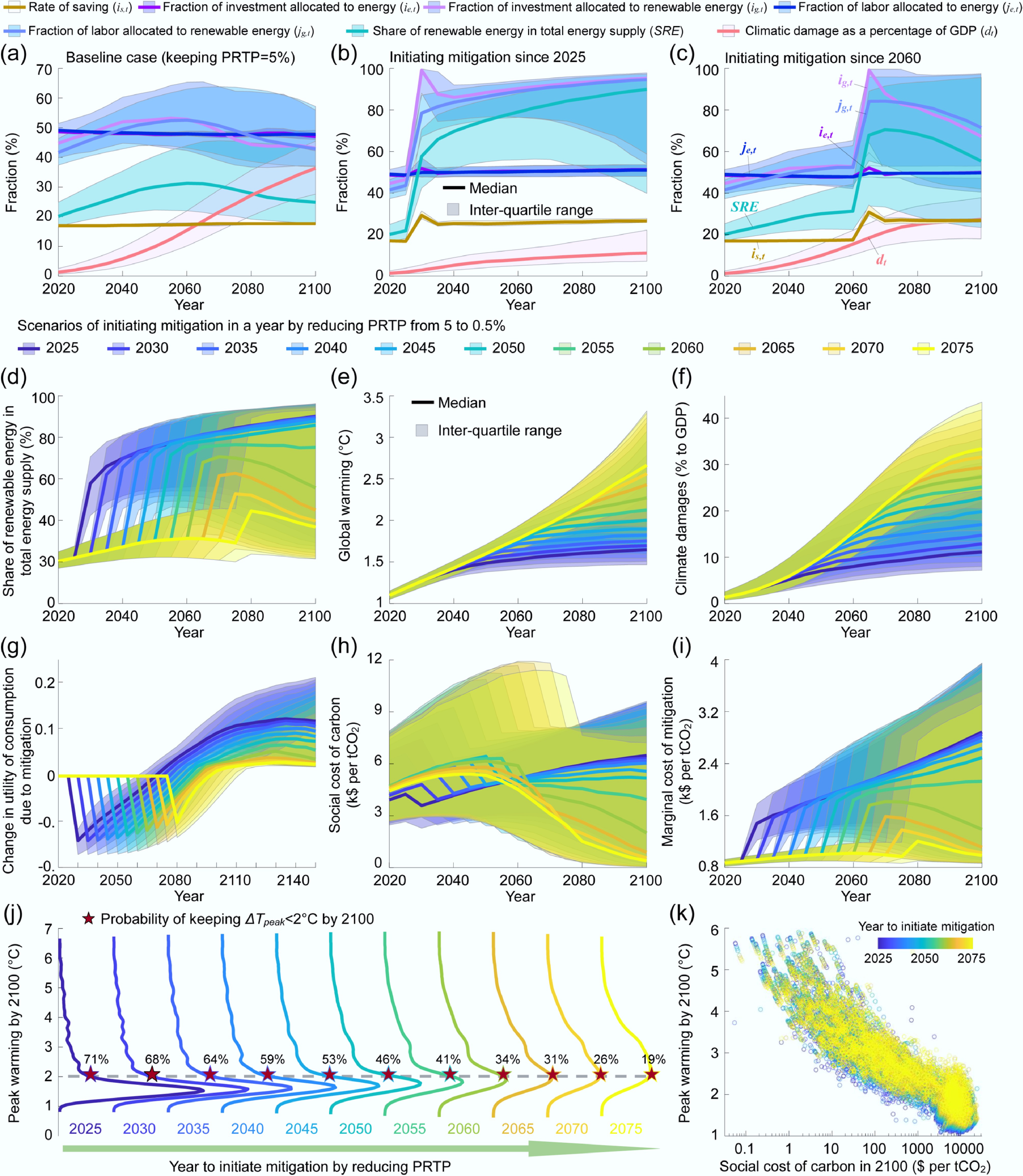
Figure 3. 

Economic and climatic impacts of initiating mitigation in a specific year. (a)−(c) Comparison of the temporal trends in the optimal rate of saving, the fraction of labor and investment allocated to produce energy and renewable energy, the share of renewable energy within total energy, and climatic damages as a percentage of GDP between the baseline scenario keeping the pure rate of time preference (PRTP) at 5% (a) and the scenario of mitigation by introducing an impulse reduction in the PRTP from 5% to 0.5% after 2025 (b) or 2060 (c). (d)–(i) Temporal trends in (d) the share of renewable energy, (e) global warming, (f) climatic damage, (g) change in the utility of consumption relative to the baseline scenario, (h) the SCC, and (i) the marginal costs of mitigation in 11 scenarios initiating mitigation in a specific year between 2025 and 2075. (j) Comparison of the probability distribution of peak warming by 2100 in 10,000 Monte Carlo simulations when mitigation is initiated in a specific year between 2025 and 2075. The probability of keeping global warming below 2 °C by 2100 is indicated by the pentagram. (k) Scatter plots of the projected global peak warming by 2100 against the SCC in 2100 in the Monte Carlo simulations. The SCC is calculated as the discounted total damages in the future caused by an increase in tCO₂ emissions at present under a PRTP of 0.5%^[42].

In the baseline case (i.e., initiating mitigation in years after 2100), the share of renewable energy (SRE) is projected to increase from ~20% in 2020 to ~30% in 2060 and then decrease to ~20% in 2100, while climatic damages are projected to increase from ~1% in 2020 to ~30% in 2100 (Fig. 3a−c). When mitigation is initiated in 2025, the SRE is projected to reach ~60% in 2030 and ~90% in 2100, whereas the predicted climatic damages amount to ~10% of GDP by 2100. In the scenario with mitigation initiated in 2060, the SRE is projected to reach ~70% in 2070 and then decrease to ~30% in 2100, whereas climatic damages are predicted to reach ~30% of GDP by 2100. When mitigation is initiated after 2060, the SRE is projected to increase slightly in response to a substantial reduction in the PRTP (Fig. 3d−f). This weak response of the SRE to mitigation is explained by the diminishing effect of mitigation in increasing the utility of consumption when mitigation is initiated after 2060, indicating that the benefits of abating CO₂ emissions can no longer effectively offset the costs of deploying renewable energy (Fig. 3g).

When strong mitigation is initiated in 2070, the SCC, as an indicator of the incentive for mitigation, is projected to decline from ~USD${\$} $6,000 per tCO₂ in 2050 to ~USD${\$} $100 per tCO₂ in 2100 (Fig. 3h). By running 10,000 Monte Carlo simulations, I predict that the probability of keeping global warming below 2 °C by 2100 would decrease from ~70% for scenarios initiating mitigation in 2025 to ~50% for scenarios initiating mitigation in 2050 and to ~20% for scenarios initiating mitigation in 2075 (Fig. 3j). On the basis of the scenarios initiating mitigation in a year between 2025 and 2075 in the Monte Carlo simulations, I observe a negative correlation between the projected peak warming by 2100 and the estimated SCC for 2100 (Fig. 3k). The probability of keeping global warming below 2 °C by 2100 is projected to be less than 10% for scenarios where the SCC in 2100 is below USD${\$} $1,000 per tCO₂.

I assume that investment and labor can be easily transferred to change the distribution of capital across sectors under welfare maximization (see Eqs. 11−16), although capital itself cannot be directly exchanged between sectors^[44]. However, the allocation of both labor and investment is subject to inertia, because time and financial investment are required to train workers moving from fossil fuel industries to sectors using renewable energy^[12]. I illustrate the impact of incorporating logistics in labor and investment on the pathway of mitigation (Supplementary Fig. S2). When considering this inertia^[12], strong mitigation needs to be further advanced to avoid a diminishing incentive for mitigation. For example, the time of initiating mitigation to avoid a declining SCC needs to be advanced from ~2050 to ~2040 if 50% of the investment entering a new sector is consumed by logistics and if worker retraining resulting from job displacement takes ~10 years. For scenarios initiating mitigation in 2050, te SRE achieved by 2150 is projected to decline from ~99% to ~30% if 90% of the investment entering a new sector is consumed by logistics, or ~40% if retraining displaced workers takes 5−15 years. More empirical studies quantifying the requirements of time and financial investment in logistics are needed to precisely predict the timing of mitigation to avoid transformative changes in the socioeconomic system.

Sensitivities of the SSC to the model's parameters

The socioeconomic tipping point is defined as an abrupt and potentially irreversible shift in the socioeconomic system induced by climate change, which is associated with potentially severe and cascading impacts on human society and economies^[55]. Most studies on climate discourse have focused on ecological and physical climate systems^[4,36−38], but little attention has been paid to examining the socioeconomic feedback^[39]. Recently, efforts have been made to fill in this gap by creating methodologies to identify and analyze socioeconomic tipping points, such as the collapse of winter tourism caused by a lack of snow, farmland abandonment caused by failures in crop production, and migration to escape coastal flooding caused by sea level rise^[55]. I modify the energy-economy model in an IAM^[44] to illustrate the socioeconomic feedback of a declining SCC on the mitigation pathway (Fig. 3). My results suggest that the incentive for mitigation might not be as persistent as expected (e.g., refs.^[16,17,35]) when mitigation is initiated in the years after 2060. In this respect, containing the transmission of COVID-19 can be considered as an analog for this socioeconomic tipping point^[55]. In that case, some governments chose to lift their controls in 2020 or 2021 to protect the economy when the risk of infection crossed a threshold, mainly because of the high economic damage caused by lockdown and the limited effects of containment^[56]. It is therefore likely that the slow deployment of renewable energy could lead to a diminishing incentive for mitigation when the damage caused by climate change cannot be recovered by abating CO₂ emissions in the short term.

To illustrate the factors influencing the timing of mitigation required to avoid crossing this socioeconomic tipping point, I compare the temporal trends of the SCC among a number of sensitivity experiments, where 10 key parameters are varied separately in the model (Fig. 4). When mitigation is initiated in the years after 2070, an abrupt decline in the SCC following an initial increase remains robust, except for scenarios involving very strong effects of technological advances (L_R > 15%), instantaneous responses of global warming to abating CO₂ emissions (τ_R < 2 years), short CO₂ lifetimes in the atmosphere (τ_L < 200 years), high thresholds of global warming for crossing catastrophic tipping points in the climate system (T₅₀ > 2.5 °C), low damage caused by crossing catastrophic climate change thresholds (d_c < 30%), high levels of damage caused by crossing catastrophic climate change thresholds (d_c > 65%), high elasticities of substitution between fossil fuels and renewable energy (σ_E > 2.5), low economic growth rates (k_p < 0.5%), high capacities of "backstop" technologies capable of abating CO₂ emissions at a cost of USD${\$} $100 per tCO₂ (B_s ≥ 2 Gt CO₂ y⁻¹)^[57], or abrupt improvements in energy-use efficiency over 2025−2050 (k_u > 5% y⁻¹). Following a decline in the SCC, global warming is projected to accelerate as a result of continued fossil fuel use and anthropogenic CO₂ emissions, driven by weak incentives for deploying expensive renewable energy (Supplementary Fig. S3).

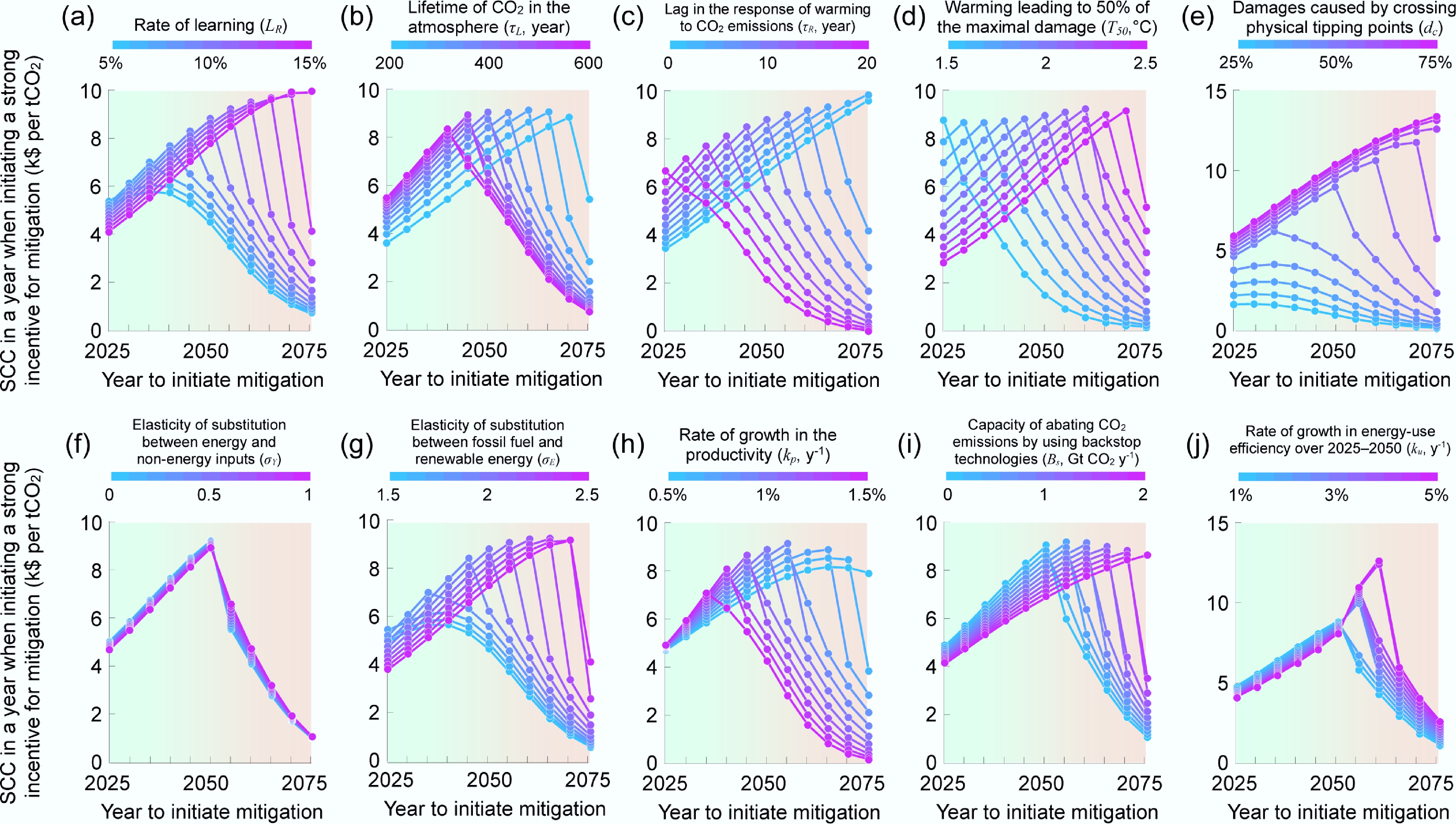
Figure 4. 

Sensitivities of the social cost of carbon (SCC) to key parameters in the model. The SCC is calculated for the year when initiating a strong incentive for mitigation in a set of sensitivity experiments which varied (a) the rate of learning (L_R), (b) the atmospheric lifetime of CO₂ (τ_L), (c) lag time of the response of global warming to CO₂ emissions (τ_R), (d) the threshold of global warming for crossing catastrophic tipping points in the climate system (T₅₀), (e) the maximal climatic damage caused by crossing catastrophic tipping points as a percentage of GDP (d_c), (f) the elasticity of substitution between energy and nonenergy inputs (σ_Y), (g) the elasticity of substitution between fossil fuels and renewable energy (σ_E), (h) the rate of growth in the productivity (k_p), (i) capacity of backstop technologies abating emissions at a cost of USD${\$} $100 per tCO₂, and (j) the abrupt increase in energy-use efficiency over 2025−2050 (k_u). The impact of varying each parameter is estimated separately while keeping the other parameters unchanged (L_R = 10%, τ_L = 400 years, τ_R = 10 years, T₅₀ = 2 °C, d_c= 50%, σ_Y = 0.5, σ_E = 2, k_p = 1% y⁻¹, B_S = 0, and k_u = 1% y⁻¹). The SCC is estimated under a PRTP of 0.5%⁴² in the optimal path under welfare maximization.

Response of global warming to initiating mitigation in a specific year

The Sixth Assessment Report of the Intergovernmental Panel on Climate Change (IPCC) employed > 100 versions of IAMs from > 50 model families to generate > 1,000 scenarios of energy transitions and global warming by representing many possible strategies of mitigation^[2]. As a feature of cost-benefit IAMs, the pathway of mitigation is optimized by evaluating the economic costs of implementing climate policies against the benefits of reducing the climatic damage (e.g., Dynamic Integrated Model of Climate and the Economy (DICE)^[46], Policy Analysis of the Greenhouse Effect (PAGE)^[32], the Climate Framework for Uncertainty, Negotiation and Distribution (FUND)^[33]). In contrast, process-based IAMs simulating interactions between human activities (e.g., energy use and land use) and environmental processes or representing characteristics of specific mitigation technologies (e.g., The Regional Model of INvestments and Development (REMIND)^[31] and Model for Energy Supply Strategy Alternatives and their General Environmental Impact (MESSAGEix)^[34]) rely on the exogenous pathways for policy scenarios and typically assume that the incentive for mitigation remain persistent over time. However, there is a lack of IAMs representing socioeconomic feedback once the incentive for mitigation declines. In this respect, characterizing the response of global warming to mitigation by accounting for the evolution of the SCC in this study provides a comparative advantage over previous IAMs considered by the IPCC^[2].

In an economically optimal pathway predicted by cost-benefit IAMs, the SCC, as an indicator ofthe incentive to reduce CO₂ emissions, could match the marginal cost of mitigation, which, in turn, determines global warming as well as the damage caused by climate change^[33,33,46]. Most cost-benefit IAMs postulate that the SCC would increase as the climatic damage increases as a result of rising temperatures^[16,17], while the costs of mitigation could decrease because of technological advances (e.g., from USD${\$} $500−1,000 to USD${\$} $100−200 per tCO₂ when abating 100% of CO₂ emissions^[16,35]). I show that the SCC might decline abruptly if a delay in mitigation exceeds a certain period. This finding is consistent with the results of simulations obtained by other IAMs when considering the impacts of catastrophic climate tipping points^[36−38]. I observe an abrupt acceleration in global warming when considering intermediate climatic damage (d_c) and initiating mitigation in a year after 2050 (Fig. 5a, d). I show that the threshold of d_c keeping global warming below 2 °C could increase as the elasticity of substitution between fossil fuels and renewable energy (σ_E) decreases or the learning rate (L_R) decreases, either of which could increase the future cost of replacing fossil fuels with renewable energy.

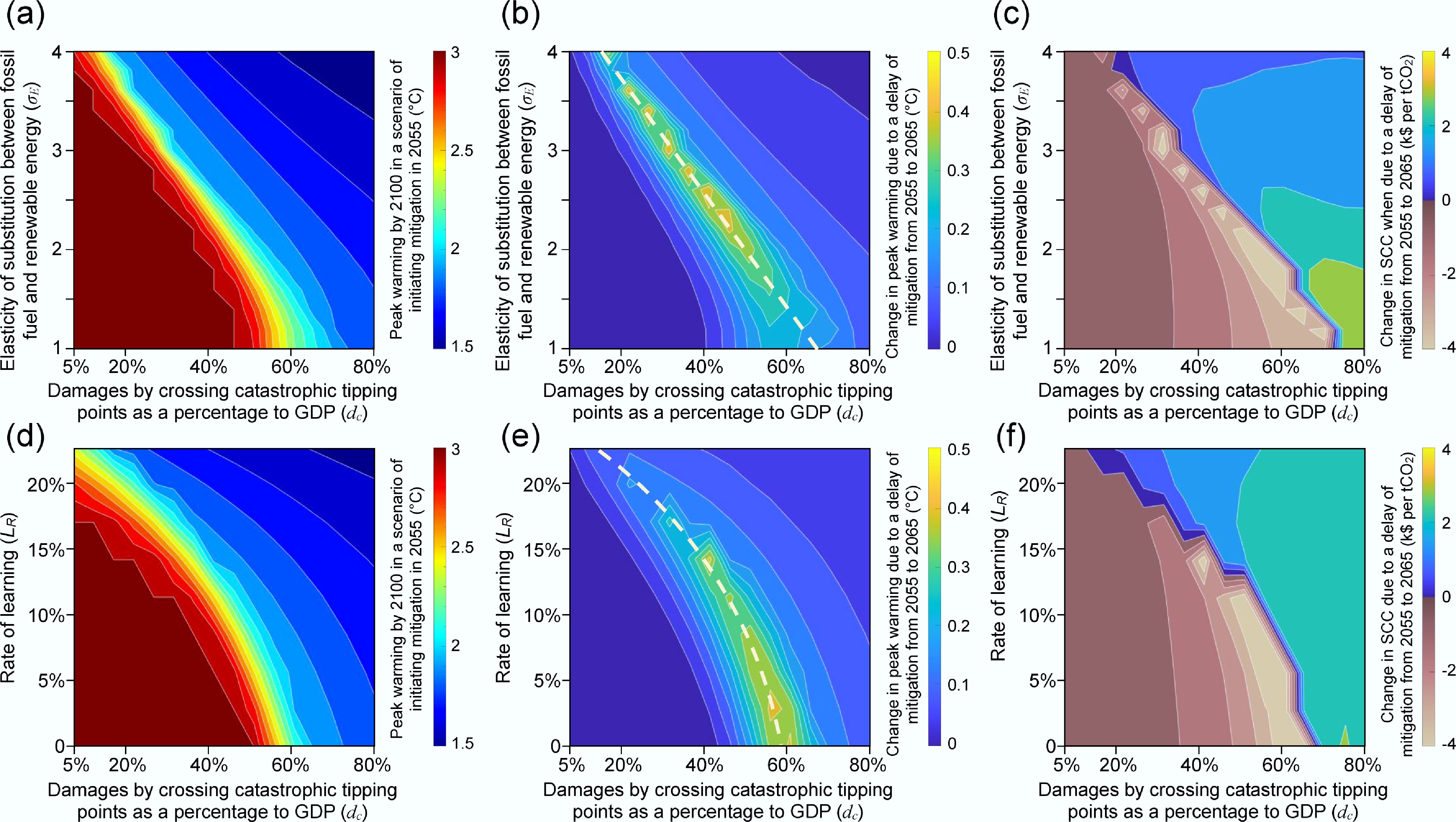
Figure 5. 

Responses in the projected peak warming by 2100 and the SCC to a delay in the year of initiating mitigation. (a) Prediction of peak warming by 2100 in scenarios initiating mitigation in 2055 when varying the elasticity of substitution between fossil fuels and renewable energy (σ_E) and the climatic damage caused by catastrophic tipping points (d_c) simultaneously. (b), (c) Responses in (b) the projected peak warming by 2100 and (c) SCC estimated for the year of initiating mitigation to a delay in the year of initiating mitigation from 2055 to 2065 when varying σ_E and d_c simultaneously. (d) Prediction of peak warming by 2100 in the scenario of initiating mitigation in 2055 when varying the rate of learning (L_R) and d_c simultaneously. (e), (f) Responses in (e) the projected peak warming by 2100 and (f) the SCC estimated for the year of initiating mitigation to a delay in the year of initiating mitigation from 2055 to 2065 when varying L_R and d_c simultaneously. Adopting a higher σ_E leads to a lower cost of replacing fossil fuels with renewable energy, whereas adopting a higher L_R leads to a faster reduction in the prices of renewable energy as a result of technological advances. The impact of varying σ_E, L_R, and d_c is examined while keeping the other parameters unchanged (L_R = 10%, τ_L = 400 years, τ_R = 10 years, T₅₀ = 2 °C, d_c = 50%, σ_Y = 0.5, σ_E = 2, k_p = 1% y⁻¹, B_S = 0, and k_u= 1% y⁻¹). The SCC is estimated under a PRTP of 0.5%^[42] in the optimal path for welfare maximization.

Further, I illustrate a range of σ_E that could lead to an acceleration in global warming when mitigation is delayed from 2025 to 2035 (Supplementary Fig. S4) or from 2055 to 2065 (Fig. 5b, e). I project that there is a transformative change in the energy−economy−climate system that is featured by an acceleration in global warming after a certain threshold of global warming is exceeded (Fig. 5c, f). Using the CES function^[45], I predict that mitigation could lead to costs that amount to ~30% (σ_E = 1), ~40% (σ_E = 2), and ~70% (σ_E = 3) of GDP in order to replace 90% of fossil fuels with renewable energy in 2025 (Fig. 2b). In contrast, the costs of mitigation are predicted to be much lower in previous IAMs (e.g., causing a GDP loss of ~5% when reducing global CO₂ emissions by 90%^[46]). A recent meta-analysis^[20] suggested that achieving net-zero CO₂ emissions in the steel and cement sectors could increase production costs by 40%−60%, which provides some support for the high costs of mitigation considered in this study.

Uncertainties in the prediction

It is valuable to forecast the decline in the incentive for mitigation as early as possible, which is challenging because of the uncertainties in prediction. Uncertainties in prediction stem from the inherent complexity of IAMs and the limitations of simulating future scenarios, including uncertainties regarding economic and population growth, technological changes, the climate system's responses, and the effectiveness of policy interventions. To illustrate uncertainties in my prediction, I performed 10,000 Monte Carlo simulations by focusing on uncertainties in the model's parameters. However, the numerical results presented in this study (e.g., the latest year of mitigation to avoid a declining SCC) should be interpreted with caution because of significant uncertainties in the model's parameters (see a summary of parameter uncertainties in Supplementary Table S2). It should also be noted that structural and technical imperfections and uncertainties in the outcomes^[58] are not quantified in this study. Addressing these uncertainties requires a pluralistic approach and risk premium methods to improve confidence in the predictions^[58]. In addition, uncertainties in key model parameters (e.g., how fast global warming responds to CO₂ emissions, how technological advances reduce the prices of renewable energy) remain significant because of a lack of data to constrain these parameters in this study. Reducing uncertainties in the key parameters requires more empirical data from observations^[43]. For example, monitoring the rate of global warming and the progress of deploying renewable energy could help us constrain the parameters in the model, enabling decision-makers to take urgent actions before crossing a socioeconomic tipping point.

I illustrate such use through a cursory study relating the temporal trend in the SCC to a potential range observed for future climatic damage or the share of renewable energy within the total energy supply. To do it, I ran 10,000 Monte Carlo simulations to predict the probability of observing a declining SCC by 2200 and the associated peak warming by 2100 by randomly varying the key parameters in this model. As expected, the range of the estimated SCC is wide, which is associated with a large spread in the temporal trend of the SCC (Fig. 6). Nevertheless, the probability of the SCC declining increases robustly in response to a delay in the year of initiating strong mitigation. For example, the probability of crossing the socioeconomic tipping point, featured by a declining SCC, is the highest when mitigation is initiated over a 5-year period centered on 2055, whereas the accumulated probability exceeds 90% when mitigation is initiated in any year between 2025 and 2075. In previous IAMs (e.g., refs^[16,17,46]), the share of renewable energy within total energy (SRE) increases continuously as climatic damage (d_t) increases. This is consistent with my result in scenarios that do not cross the socioeconomic tipping point, i.e., when a strong mitigation incentive is initiated before 2050, where the average SRE increases from ~80% to ~90% as d_t increases from ~10% to ~20% of GDP (Fig. 6b). In contrast, the average SRE rises slightly as d_t increases from ~10% to ~20% in scenarios that cross the socioeconomic tipping point, i.e., when a strong mitigation incentive is initiated after 2050 (Fig. 6c). When d_t surpasses 10% in a specific year, the probability of SRE > 60% is very high in scenarios without crossing the socioeconomic tipping point. In contrast, for scenarios with a declining SCC, the probability of SRE > 60% could be significantly reduced when d_t surpasses 10% in a specific year. Therefore, observation of a low SRE when d_t surpasses a threshold may serve as an early warning signal of a declining SCC, indicating that stronger mitigation policies are needed to accelerate deployment of renewable energy.

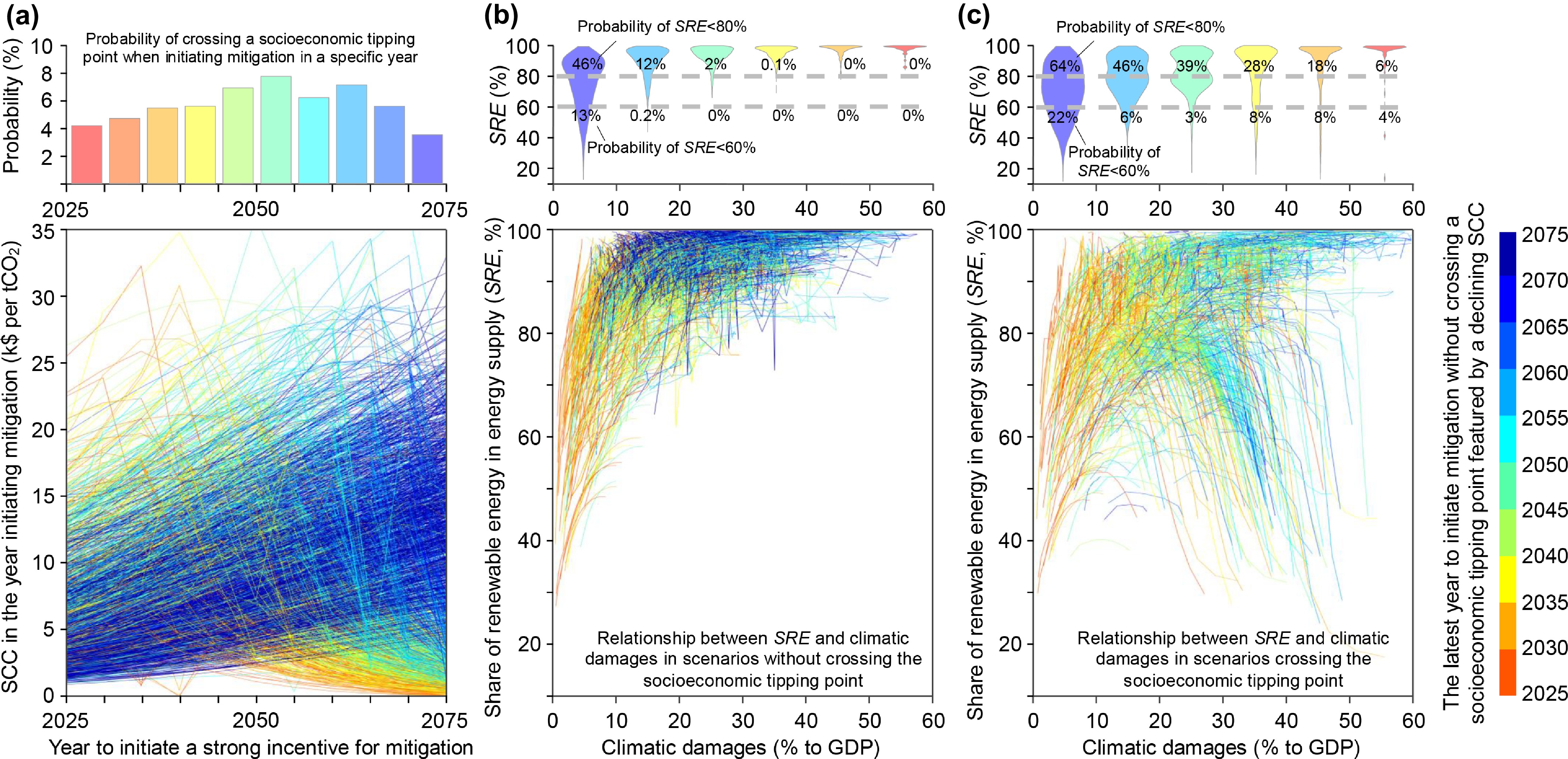
Figure 6. 

Relationships between the share of renewable energy within total energy (SRE) and the projected climatic damage. (a) Comparison of the trend in the SCC estimated for the year of initiating a strong incentive for mitigation across 10,000 Monte Carlo simulations. The line color denotes the latest year of initiating a strong incentive for mitigation without crossing a socioeconomic tipping point featured by a declining SCC in the Monte Carlo simulations. The bar plot shows the probability of crossing this tipping point when mitigation is initiated within a 5-year period. (b) Relationship between SRE and climatic damage in scenarios without crossing a socioeconomic tipping point. (c) Relationship between SRE and climatic damage in scenarios crossing the socioeconomic tipping point featured by a declining SCC. In (b) and (c), the violin plot shows the probability of SRE based on the range of climatic damage in a future year.

The high costs of accelerating the deployment of renewable energy to achieve an energy system with net-zero CO₂ emissions in the short term, combined with the uncertain long-term outcomes of climate mitigation, lead to hesitance about immediately stopping the use of fossil fuel at present^[17−19]. Extending the period of fossil fuel use reduces the probability of meeting the Paris Agreement targets for limiting global warming below 1.5 or 2 °C^[2]. Given the observed damage caused by climate change^[27−30], the recent growth in global anthropogenic CO₂ emissions^[5,15] indicates that current mitigation is likely to deviate from the optimal pathway for meeting the targets of the Paris Agreement^[17−19]. To clarify the potential impact of deferring the time of initiating a strong incentive for mitigation, I account for the effect of socioeconomic feedback on mitigation by optimizing the intertemporal decisions regarding both consumption behavior and the allocation of labor and investment between sectors relying on fossil fuels and renewable energy under welfare maximization in a modified cost-benefit IAM^[43]. I show that, in response to continuously rising temperatures, the SCC might increase initially but then decrease once the climatic damage surpasses a threshold, leading to a declining incentive for mitigation and thus accelerated global warming.

The impact of varying the parameters in the IAM on the trend of the SCC suggests that crossing the socioeconomic tipping point, featured by a declining SCC, might be irreversible unless noneconomic instruments are implemented immediately to accelerate mitigation, which makes this socioeconomic tipping point distinct from physical tipping points in the climate system that have been considered by previous studies^[36,37]. The latest year of initiating a strong incentive for mitigation to avoid crossing this socioeconomic tipping point could be affected by altering the choice of parameters in the IAM, but a high probability of crossing this socioeconomic tipping point when delaying mitigation to years after 2050 remains robust. Considering uncertainties in the model's parameters by running Monte Carlo simulations, I demonstrate a low share of renewable energy within the total energy supply when the observed climatic damage surpasses a threshold (e.g., ~10% or ~20% of GDP). This could form an early warning signal of crossing the socioeconomic tipping point, which is featured by a declining SCC and thus a diminishing incentive for mitigation.

Climatic damages have amounted to ~USD${\$} $240 billion in 2024 when accounting for the impacts of severe climate events, including convective storms in the United States; floods in the southern and central regions of China, Brazil, and Europe; Typhoon Yagi; Hurricane Milton; and heat waves in South Asia (e.g., Bangkok's heat index hit 52 °C in April)^[59]. I propose developing an early warning system to forecast the SCC and the incentive for mitigation. The 28^th United Nations Climate Change Conference (COP28) aims to shift the world's first Global Stocktake to increasing ambition and accelerating inclusive and just actions of mitigation, calling for instruments to monitor and evaluate the real-world progress of energy transitions^[60]. After COP28, legislation is urgently needed to boost global actions aimed at stopping the use of fossil fuels to meet the targets of the Paris Agreement^[15]. According to this study, the damage caused by climate change and the progress of deploying renewable energy could be simultaneously monitored to forecast the probability of crossing a socioeconomic tipping point in an early warning system, which could be implemented in the Global Stocktake of the Paris Agreement (Fig. 6). Ultimately, this will allow decision-makers to take urgent actions before crossing the socioeconomic tipping point and avoid unexpected, irreversible, and dangerous climate change.